Foundations of
Data Science

Spring 2026 | Data 2 (399)
Jeffrey M. Girard | Lecture 04a

Roadmap

  • Learn the principles of data storage and the tidy data format

  • Read data from and write data to comma-separated values files

Principles

Tidy Data Principles

  • There are many ways to store data
  • We will be learning the tidy data format
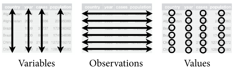
    • Data should be rectangular
    • Each variable has its own column
    • Each observation has its own row
    • Each value has its own cell

Other Data Advice

  • Name all variables in the first row
    • This is called a header row
  • Avoid merged cells for data storage
    • These are okay for communication
  • Avoid empty cells whenever possible
    • Mark missing data as NA
  • Avoid formatting-as-data for storage
    • e.g., non-redundant color-coding

Tidying Example 1

Not Tidy

Name Ann Bob Cat Dom
Age 13 10 11 11
Weight 56.4 46.8 41.3 43.3

❌ Here, each row is a variable and each column is an observation.

Tidy

Name Age Weight
Ann 13 56.4
Bob 10 46.8
Cat 11 41.3
Dom 11 43.3

✔️ Here, each column is a variable and each row is an observation.

Tidying Example 2

Not Tidy

Names: Ann Bob Cat Dom
Age Weight
13 56.4
10 46.8
11 41.3
11 43.3

❌ Here, we have data that is not rectangular because the Names variable has its own row.

Tidy

Name Age Weight
Ann 13 56.4
Bob 10 46.8
Cat 11 41.3
Dom 11 43.3

✔️ Here, we have made the data rectangular by moving the Names variable to its own column.

Tidying Example 3

Not Tidy

country year cases / population
Afghanistan 1999 NA / 19987071
2000 2666 / 20595360
Brazil 1999 37737 / 172006362
2000 80488 / 174504898
China 1999 212258 / 1272915272
2000 213766 / 1280428583

❌ Here, we have merged cells and two values stored in a single cell.

Tidy

country year cases population
Afghanistan 1999 NA 19987071
Afghanistan 2000 2666 20595360
Brazil 1999 37737 172006362
Brazil 2000 80488 174504898
China 1999 212258 1272915272
China 2000 213766 1280428583

✔️ Here, we have un-merged the countries and separated the cases and populations variables into columns.

Tidying Example 4

Not Tidy

student grade
Amber 91.5 A-
Bristol 86.2 B
Charlene 94.0 A
Diego 89.3 B+
Legend: Psych. Major, Psych. Minor

❌ Here, we have a missing variable name and formatting-as-data.

Tidy

student psych grade letter
Amber major 91.5 A-
Bristol minor 86.2 B
Charlene major 94.0 A
Diego NA 89.3 B+

✔️ Here, we have added a column for the psych variable, removed the legend, and named the letter variable.

Tidying Example 5

Not Tidy

student grade letter
Amber 91.5 A-
Bristol* 94.2 A
Class Summary
As 2 Yay!
Bs 0
*Grade was revised.

❌ Here, we have two types of data in one file and a footnote as data.

Tidy

student grade letter revised
Amber 91.5 A- FALSE
Bristol 94.2 A TRUE
letter count notes
A 2 Yay!
B 0

✔️ Here, we have split the data into two separate tables and added the revised and notes variables.

Data Files

Data Files

  • Data is usually stored in data files
    • Importing files into R is called reading
    • Exporting files from R is called writing
  • A convenient data file type is a CSV
    • This stands for comma-separated values
    • A CSV file is easy to share with other people
  • The tidyverse package can read/write CSVs
    • The data will be stored in R as a tibble object
    • Other packages can read/write other file types

Tibbles

  • R works particularly well with tidy data
  • We store tidy data in data frames or tibbles
    • Tibbles are just fancier data frames
      (i.e., they have a few extra features)
  • To use tibbles, we need the tidyverse package
  • Tibbles are constructed from one or more vectors
    • The vectors must have the same length
    • They can contain different types of data

Reading a CSV file into R

library(tidyverse)
pdata <- read_csv("penguindata.csv") # Available on website
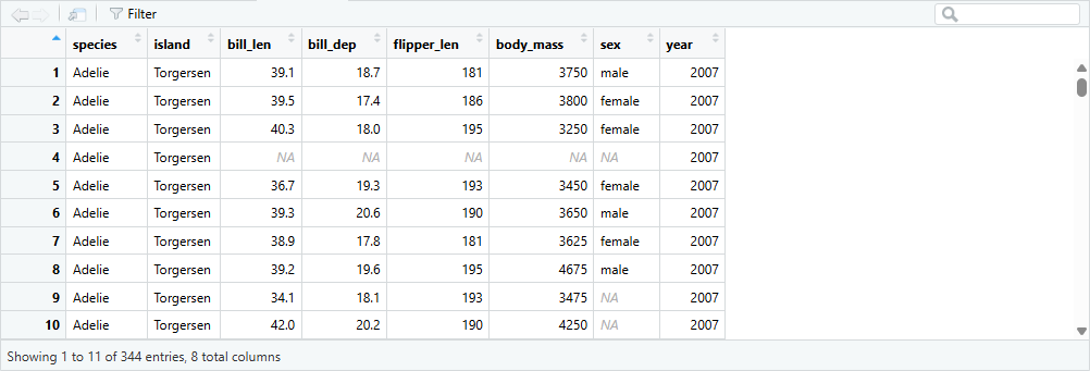
pdata
# A tibble: 344 × 8
   species island    bill_len bill_dep flipper_len body_mass sex     year
   <chr>   <chr>        <dbl>    <dbl>       <dbl>     <dbl> <chr>  <dbl>
 1 Adelie  Torgersen     39.1     18.7         181      3750 male    2007
 2 Adelie  Torgersen     39.5     17.4         186      3800 female  2007
 3 Adelie  Torgersen     40.3     18           195      3250 female  2007
 4 Adelie  Torgersen     NA       NA            NA        NA <NA>    2007
 5 Adelie  Torgersen     36.7     19.3         193      3450 female  2007
 6 Adelie  Torgersen     39.3     20.6         190      3650 male    2007
 7 Adelie  Torgersen     38.9     17.8         181      3625 female  2007
 8 Adelie  Torgersen     39.2     19.6         195      4675 male    2007
 9 Adelie  Torgersen     34.1     18.1         193      3475 <NA>    2007
10 Adelie  Torgersen     42       20.2         190      4250 <NA>    2007
# ℹ 334 more rows

Get the gist of the data with glimpse

# This shows the first few values in each column (chr=strings, dbl=numbers)
glimpse(pdata)
Rows: 344
Columns: 8
$ species     <chr> "Adelie", "Adelie", "Adelie", "Adelie", "Adelie", "Adelie"…
$ island      <chr> "Torgersen", "Torgersen", "Torgersen", "Torgersen", "Torge…
$ bill_len    <dbl> 39.1, 39.5, 40.3, NA, 36.7, 39.3, 38.9, 39.2, 34.1, 42.0, …
$ bill_dep    <dbl> 18.7, 17.4, 18.0, NA, 19.3, 20.6, 17.8, 19.6, 18.1, 20.2, …
$ flipper_len <dbl> 181, 186, 195, NA, 193, 190, 181, 195, 193, 190, 186, 180,…
$ body_mass   <dbl> 3750, 3800, 3250, NA, 3450, 3650, 3625, 4675, 3475, 4250, …
$ sex         <chr> "male", "female", "female", NA, "female", "male", "female"…
$ year        <dbl> 2007, 2007, 2007, 2007, 2007, 2007, 2007, 2007, 2007, 2007…

Dig deeper into the data with View

# This display is read-only. Data editing should be done by code, not by hand!
View(pdata)

Accessing data from a package

# Let's open the msleep data from the ggplot2 package
data("msleep", package = "ggplot2")
# Let's glimpse the tibble to learn about it
glimpse(msleep)
Rows: 83
Columns: 11
$ name         <chr> "Cheetah", "Owl monkey", "Mountain beaver", "Greater shor…
$ genus        <chr> "Acinonyx", "Aotus", "Aplodontia", "Blarina", "Bos", "Bra…
$ vore         <chr> "carni", "omni", "herbi", "omni", "herbi", "herbi", "carn…
$ order        <chr> "Carnivora", "Primates", "Rodentia", "Soricomorpha", "Art…
$ conservation <chr> "lc", NA, "nt", "lc", "domesticated", NA, "vu", NA, "dome…
$ sleep_total  <dbl> 12.1, 17.0, 14.4, 14.9, 4.0, 14.4, 8.7, 7.0, 10.1, 3.0, 5…
$ sleep_rem    <dbl> NA, 1.8, 2.4, 2.3, 0.7, 2.2, 1.4, NA, 2.9, NA, 0.6, 0.8, …
$ sleep_cycle  <dbl> NA, NA, NA, 0.1333333, 0.6666667, 0.7666667, 0.3833333, N…
$ awake        <dbl> 11.9, 7.0, 9.6, 9.1, 20.0, 9.6, 15.3, 17.0, 13.9, 21.0, 1…
$ brainwt      <dbl> NA, 0.01550, NA, 0.00029, 0.42300, NA, NA, NA, 0.07000, 0…
$ bodywt       <dbl> 50.000, 0.480, 1.350, 0.019, 600.000, 3.850, 20.490, 0.04…

Writing data from R to a CSV file

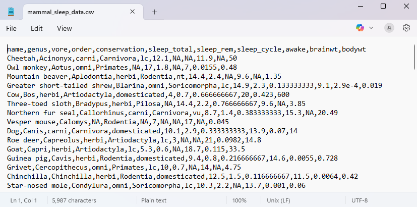
# Let's export this data so we can email it to someone without R
write_csv(msleep, file = "mammal_sleep_data.csv")