Foundations of
Data Science

Spring 2026 | Data 2 (399)
Jeffrey M. Girard | Lecture 05a

Roadmap

• Learn the principles that govern data visualization

• Create and save scatterplots using ggplot() and ggsave()

Principles

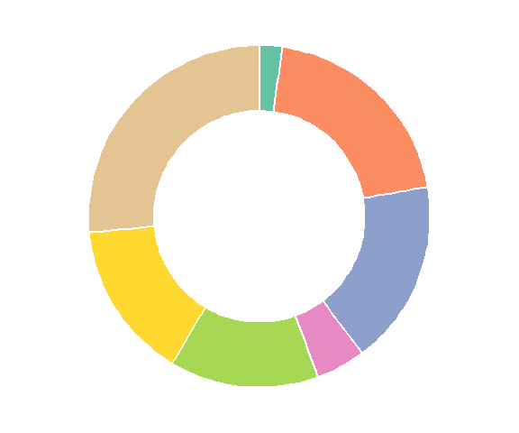
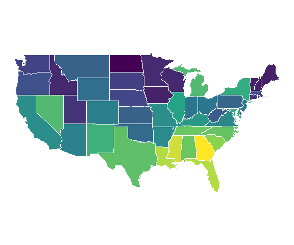
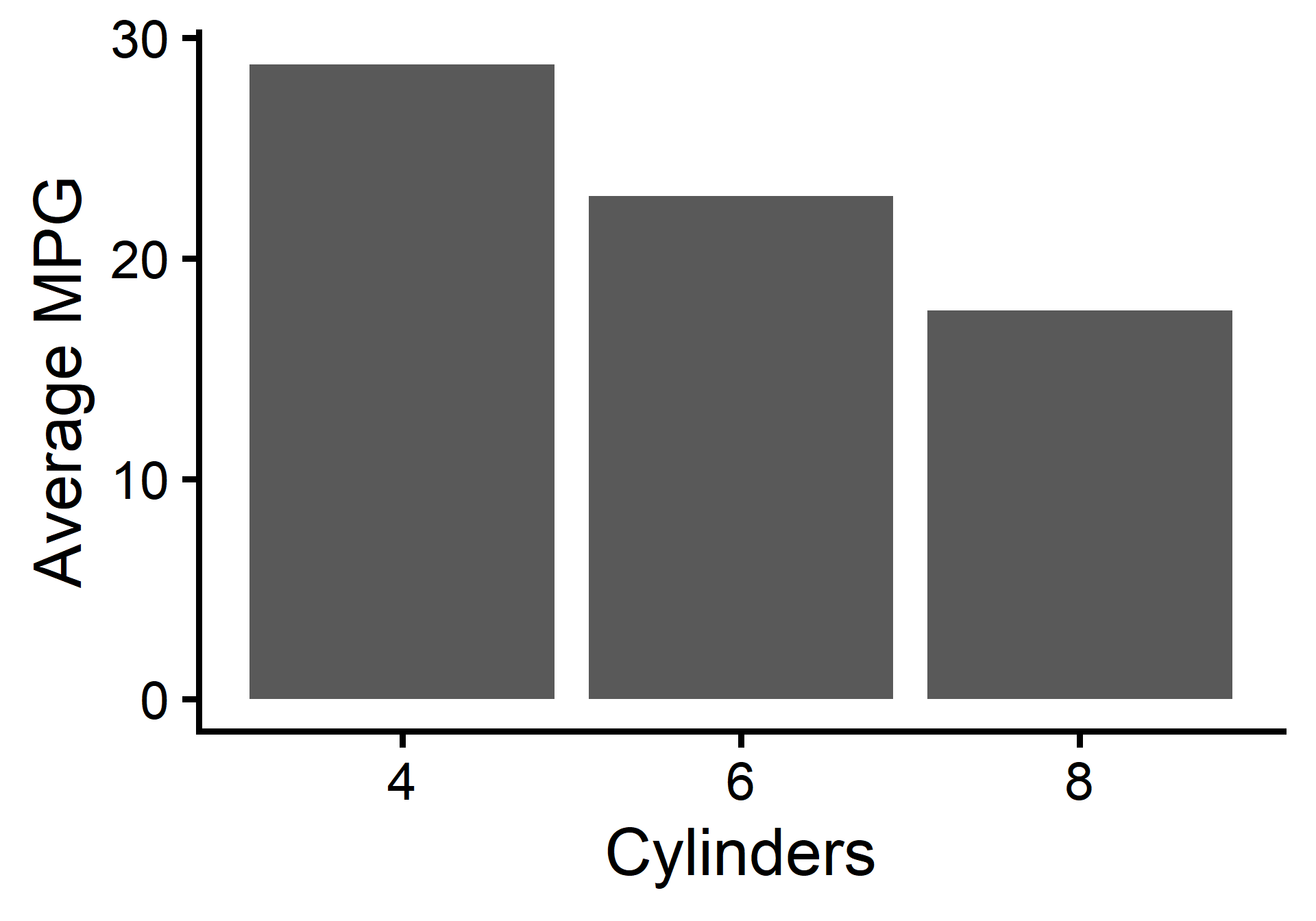
What is a graphic?

A data visualization expresses data through visual aesthetics.

Describing Graphics

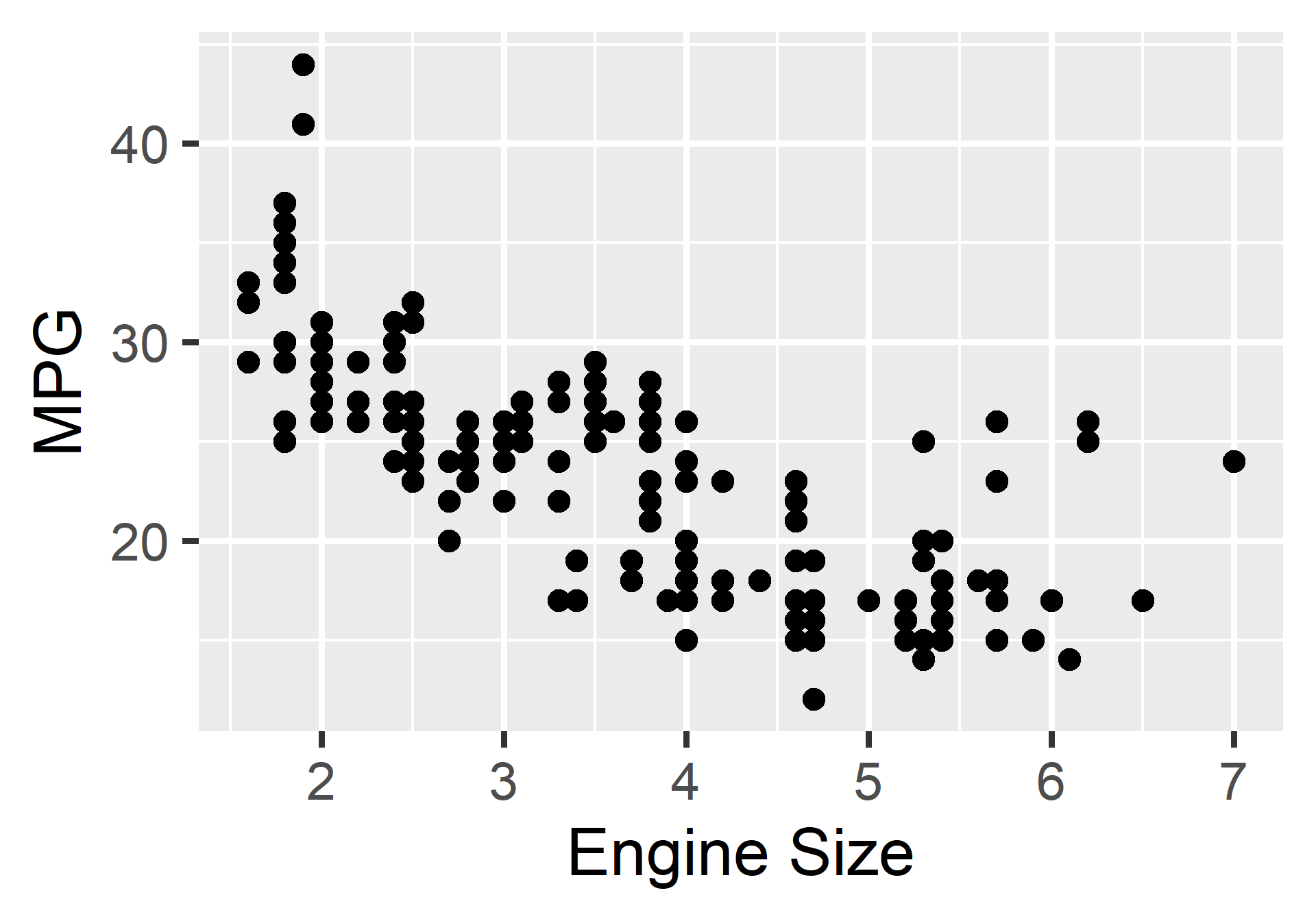
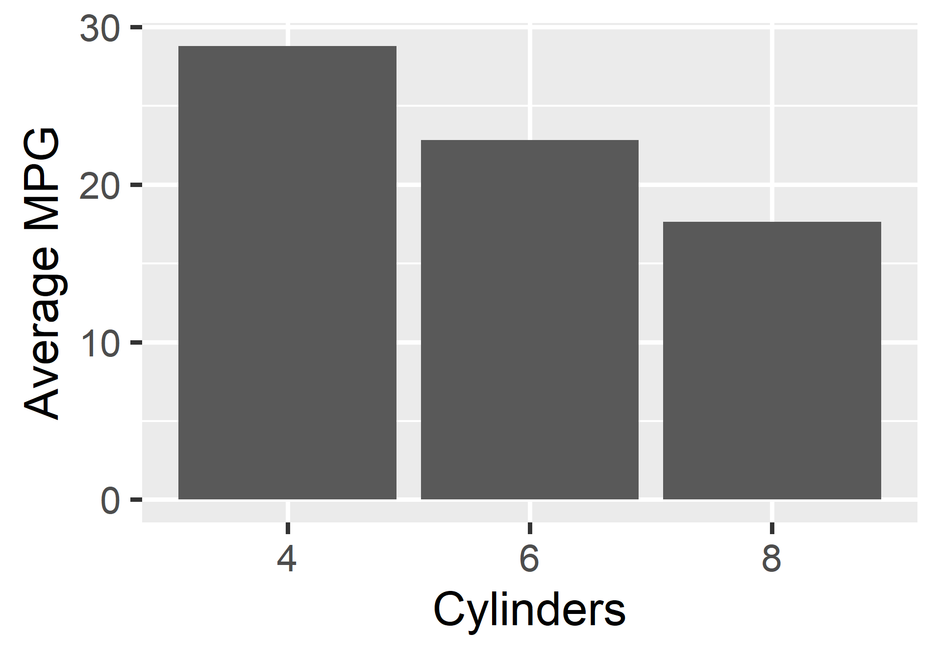
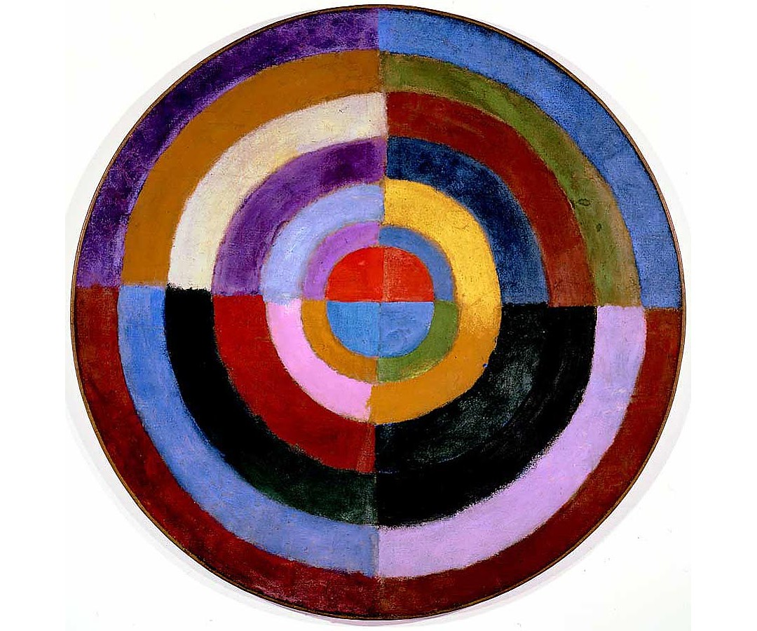
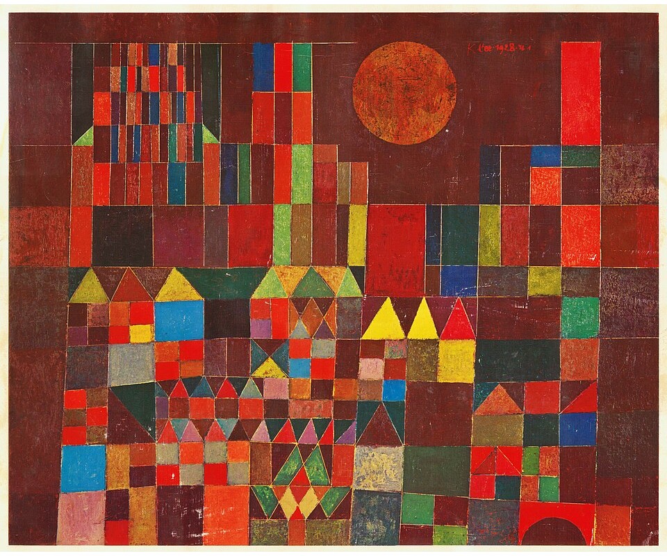
Some simple graphics are easy to describe and may even have ready names.

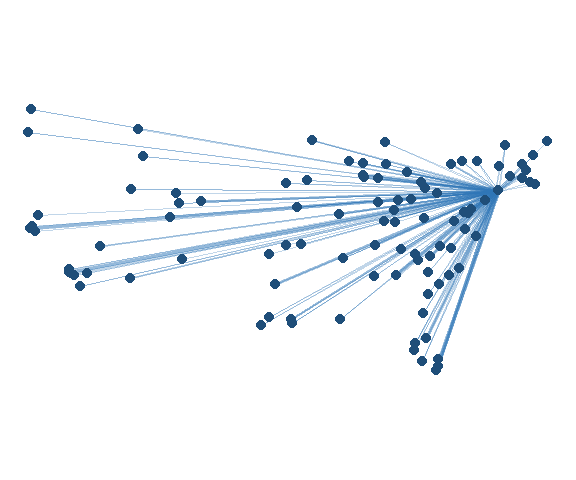
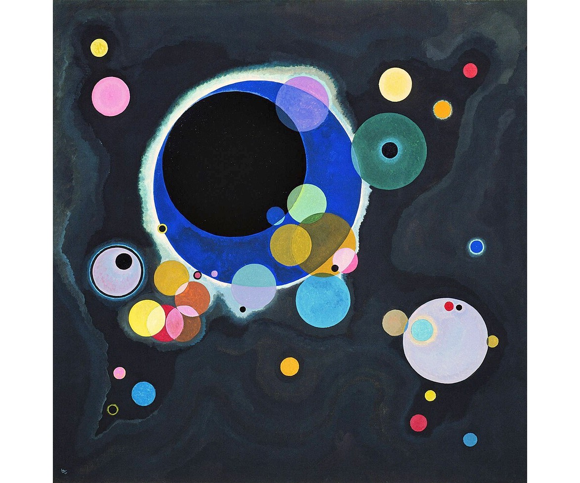
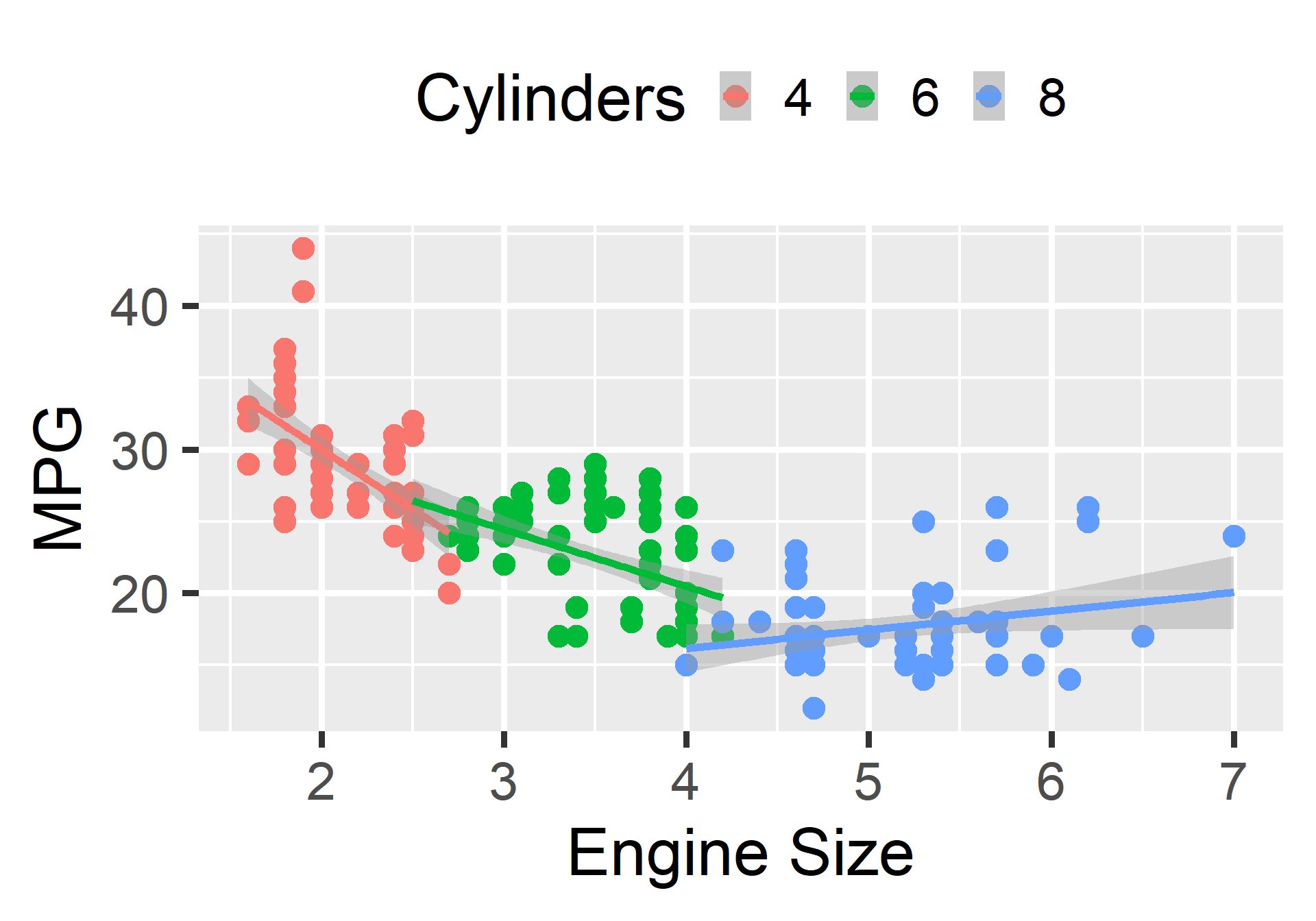
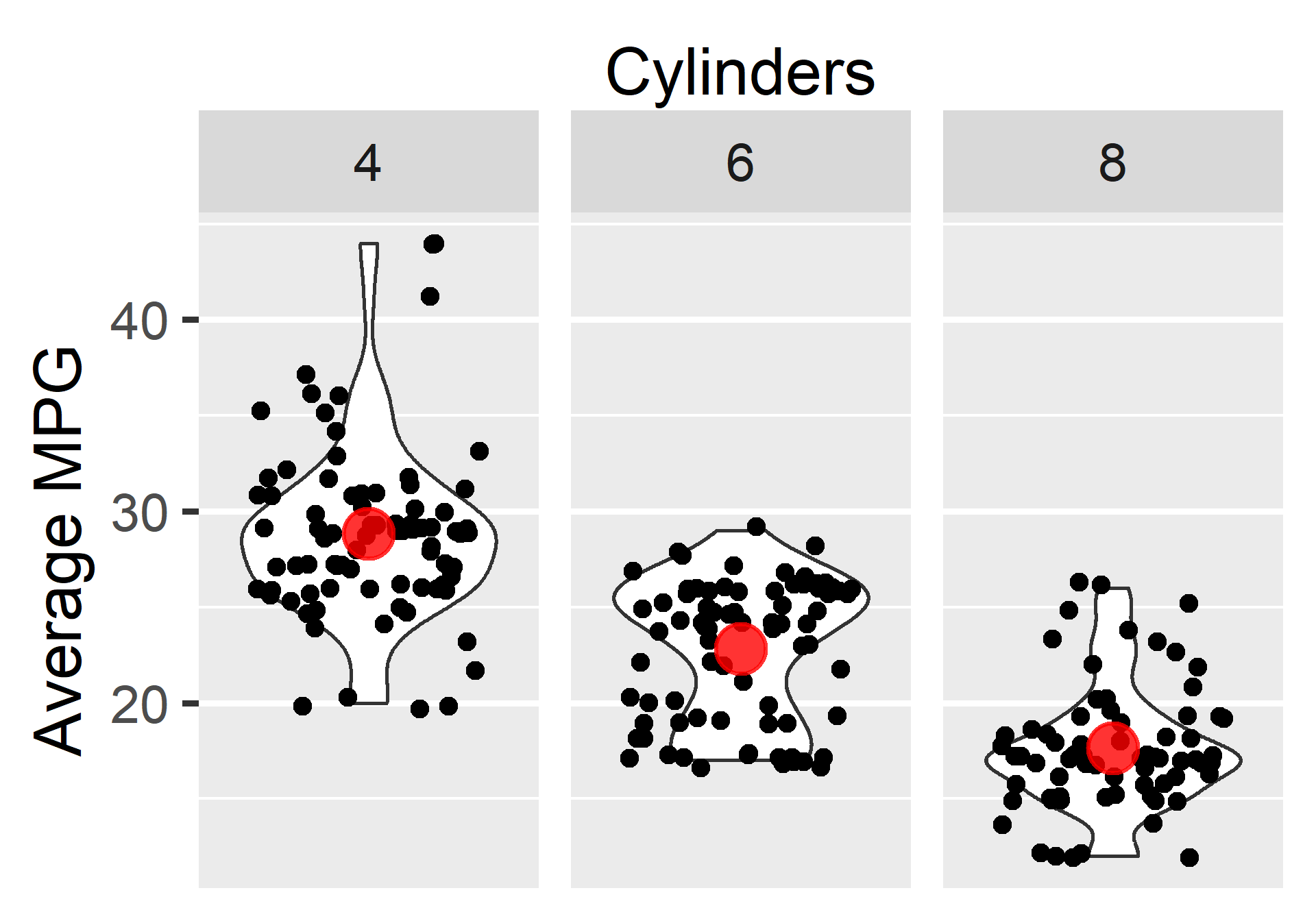
Describing Graphics

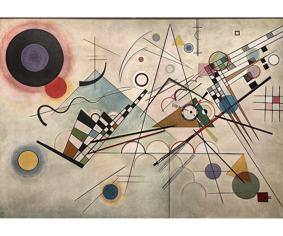
A grammar of graphics will help us describe more complex graphics.

The Grammar of Graphics

• The grammar of graphics is a set of rules for describing and creating data visualizations

• To make our data visual (and therefore put our highly evolved occipital lobes to work)…
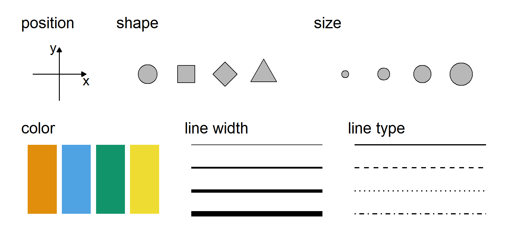
  • We connect variables to visual qualities
  • We represent observations as visual objects

• This requires four fundamental elements
  • We will first learn about them in lecture
  • We will then apply them in R using {ggplot2}

Data

data("mpg", package = "ggplot2")
mpg

# A tibble: 234 × 11
   manufacturer model      displ  year   cyl trans drv     cty   hwy fl    class
   <chr>        <chr>      <dbl> <int> <int> <chr> <chr> <int> <int> <chr> <chr>
 1 audi         a4           1.8  1999     4 auto… f        18    29 p     comp…
 2 audi         a4           1.8  1999     4 manu… f        21    29 p     comp…
 3 audi         a4           2    2008     4 manu… f        20    31 p     comp…
 4 audi         a4           2    2008     4 auto… f        21    30 p     comp…
 5 audi         a4           2.8  1999     6 auto… f        16    26 p     comp…
 6 audi         a4           2.8  1999     6 manu… f        18    26 p     comp…
 7 audi         a4           3.1  2008     6 auto… f        18    27 p     comp…
 8 audi         a4 quattro   1.8  1999     4 manu… 4        18    26 p     comp…
 9 audi         a4 quattro   1.8  1999     4 auto… 4        16    25 p     comp…
10 audi         a4 quattro   2    2008     4 manu… 4        20    28 p     comp…
# ℹ 224 more rows

Graphics require data (e.g., tibbles), which describe observations using variables.

Aesthetic Mappings

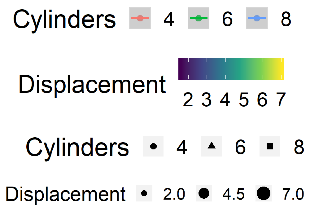
Graphics require aesthetic mappings, which connect data variables to visual qualities.

Scales

Graphics require scales, which connect specific data values to specific aesthetic values.

Geometric Objects

Graphics require geometric objects (geoms), which represent the observations.

Scatterplots

ggplot2 Basics

• The ggplot2 package is a part of tidyverse
  • No need to install or load it separately
  • It plays nicely with tibbles and wrangling

• It implements the grammar of graphics in R
  • The “gg” stands for “grammar of graphics”
  • Thus, it lets us control all four elements

• We will create a pseudo-pipeline of commands
  • However, we will use + rather than |>
  • This is because {ggplot2} predates the R pipe

Starting with data

library(tidyverse)

# CHECKLIST:
# [x] Element 1: data
# [ ] Element 2: mapping
# [ ] Element 3: scales (for free)
# [ ] Element 4: geoms

p <- 
  ggplot(
    data = mpg
  )
p

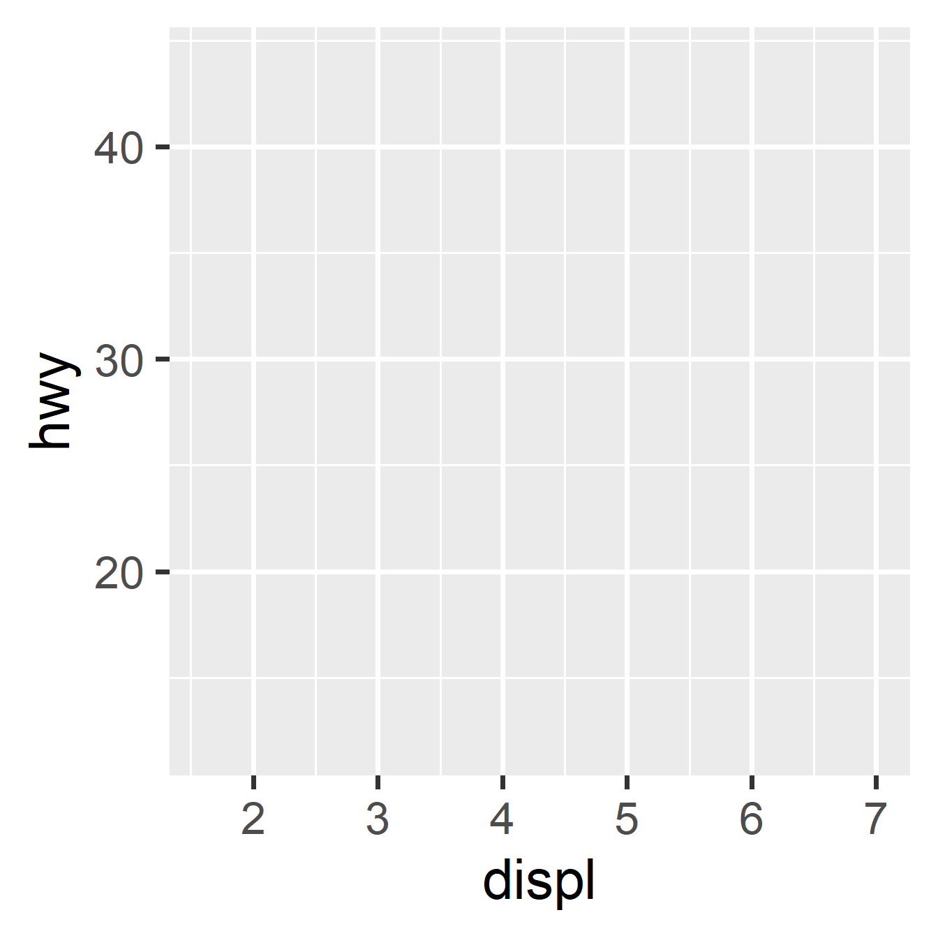
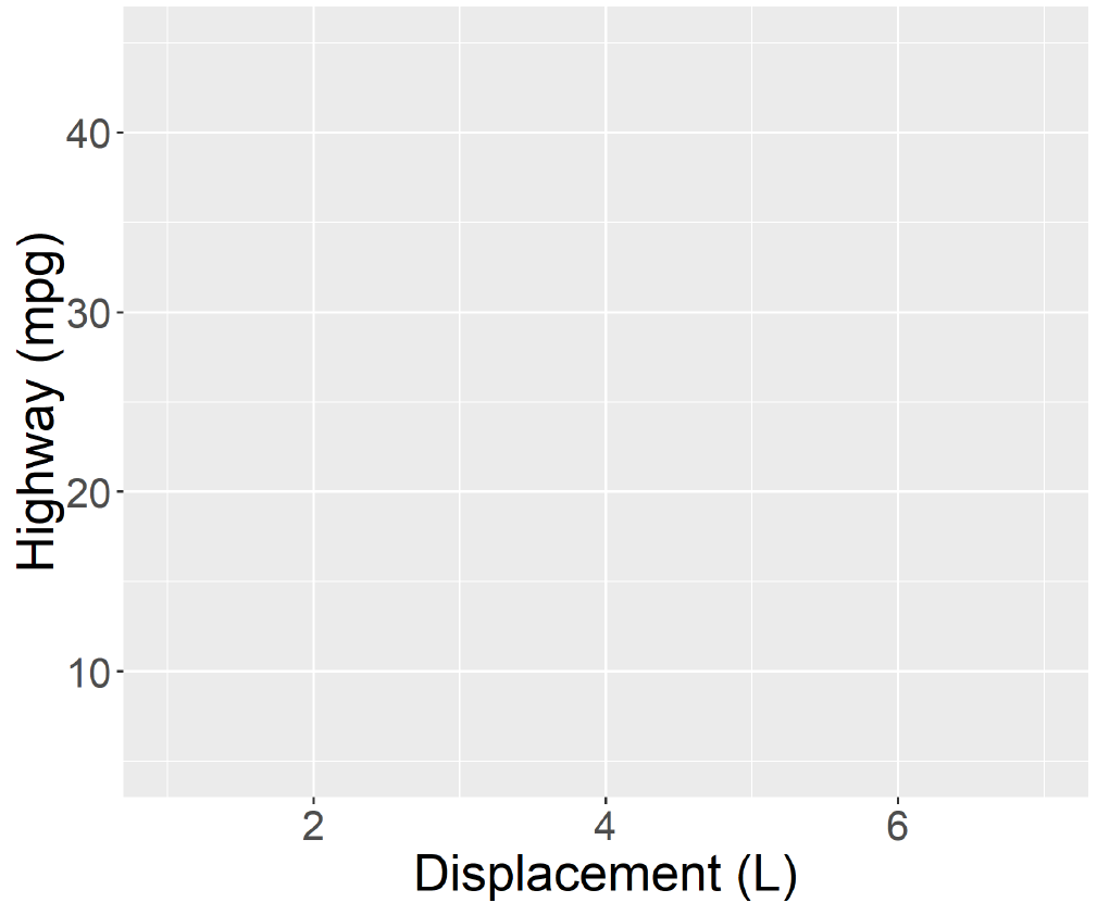
Adding aesthetic mapping

# CHECKLIST:
# [x] Element 1: data
# [x] Element 2: mapping
# [x] Element 3: scales (for free)
# [ ] Element 4: geoms

p <- 
  ggplot(
    data = mpg,
    mapping = aes(x = displ, y = hwy)
  )
p

Adding geometric objects

# CHECKLIST:
# [x] Element 1: data
# [x] Element 2: mapping
# [x] Element 3: scales (for free)
# [x] Element 4: geoms

p <- 
  ggplot(
    data = mpg,
    mapping = aes(x = displ, y = hwy)
  ) +
  geom_point()
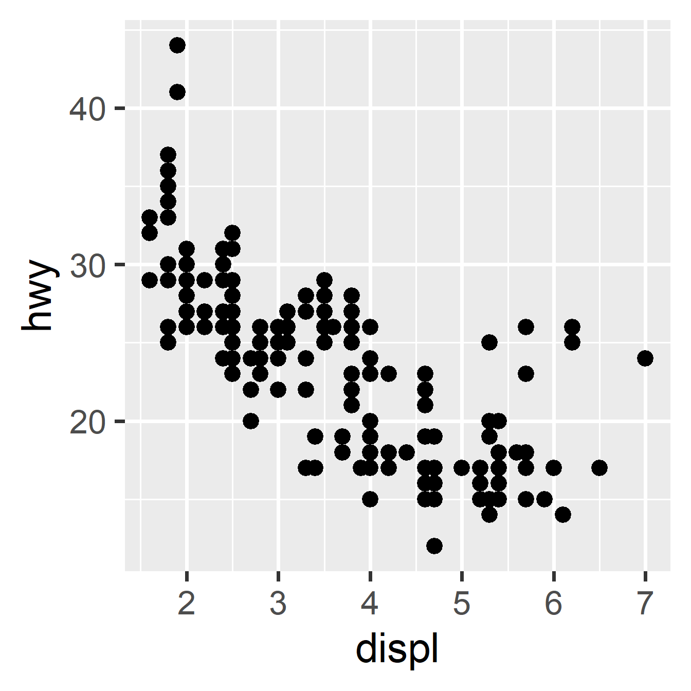
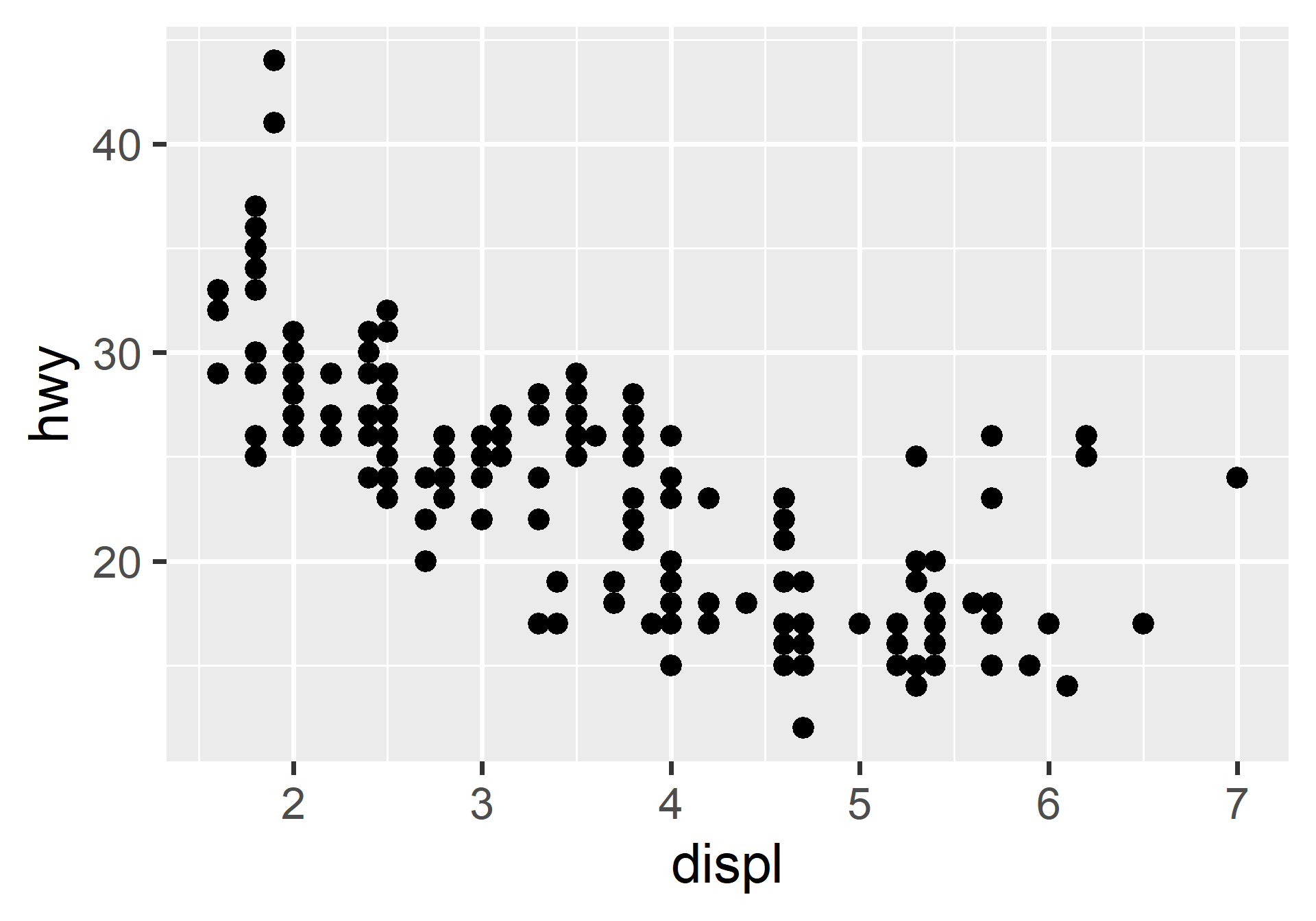
p

Compact (Positional) Coding

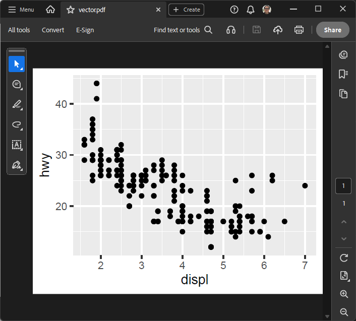
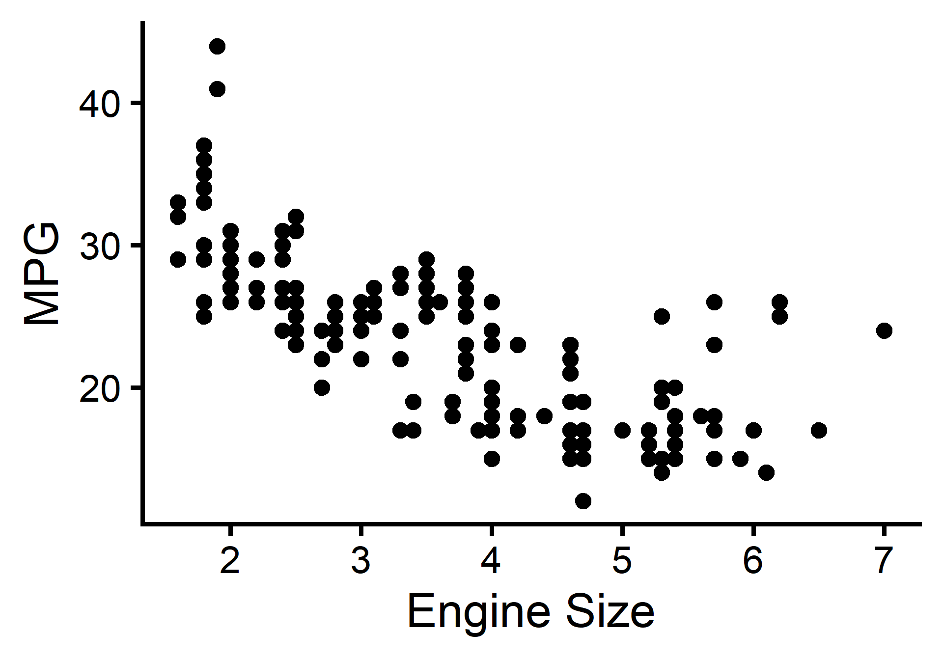
ggplot(mpg, aes(x = displ, y = hwy)) + geom_point()

Saving Graphics

Saving Graphics

• ggsave() exports ggplots to files
  • We control the exact size and format

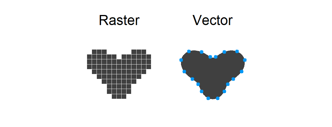
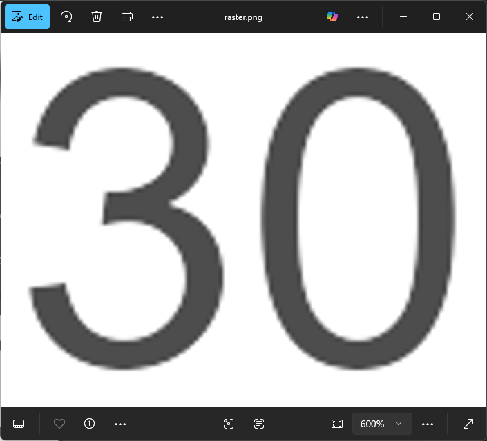
• Raster (png, jpg, bmp, tif): Compatibility

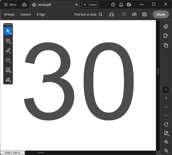
• Vector (pdf, svg, wmf, eps): Scalability

Using the ggsave function

# Prepare a graphic and assign it to an object (p)
p <- ggplot(mpg, aes(x = displ, y = hwy)) + geom_point()

# Save to a raster (png) file
ggsave(
  filename = "raster.png",
  plot = p,
  width = 9,
  height = 7,
  units = "in"
)

# Save to a vector (pdf) file
ggsave(
  filename = "vector.pdf",
  plot = p,
  width = 9,
  height = 7,
  units = "in"
)

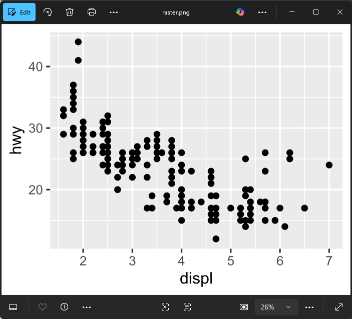
Comparing the output (full size)

raster.png - 172.1 KB

vector.pdf - 11.2 KB

Comparing the output (zoomed in)

raster.png - 172.1 KB

vector.pdf - 11.2 KB