Foundations of
Data Science

Spring 2026 | Data 2 (399)
Jeffrey M. Girard | Lecture 06a

Roadmap

Style your code to improve organization and clarity
Manage the behavior of individual code chunks in Quarto

Code Style

Style describes optional changes
- e.g., how to name files and objects
- e.g., where to add spaces and line breaks

There is no “right” or “wrong” with style

But using a consistent code style has benefits
- Code becomes more readable and predictable
- Collaboration becomes easier and smoother

We will learn about the tidyverse style guide

File Names

File names should be meaningful and clear
- models.qmd ➔ dissertation_study2_models.qmd

Avoid special characters in names (arguably this includes spaces)
- M@$teR$ Th3s1s.r ➔ masters_thesis.R

If your files need to be run in order, prefix with numbers
- 1_import.qmd, 2_model.qmd, 3_visualize.qmd

Use zero-padding as necessary (to sort them properly)
- 01_download.qmd, 02_tidy.qmd, …, 10_visualize.qmd

Sectioning and Comments

Use sections and subsections to give the file internal structure
Load all packages together at the top of the document
Use comments to explain the “why” (not the “what” or “how”)

Object Naming

Object names should use a single and consistent style
- countydata and plot_county
- Snake Case: county_data and county_plot
- Camel Case: countyData and countyPlot

Use brief, descriptive noun phrases for object names
- x ➔ heart_rate
- df ➔ aim1_data

Avoid reusing names of base R objects and functions
- e.g., F, T, c, mean, sum, pi, data

Spacing

Put spaces around most operators (arithmetic, relational, and logical)
- 1/2+3*4-5 ➔ 1 / 2 + 3 * 4 - 5
- a>3&b<=0 ➔ a > 3 & b <= 0

But don’t put spaces around “high priority” operators
- 5 ^ 2 ➔ 5^2
- ( 1 + 2 ) * 3 ➔ (1 + 2) * 3
- sum ( sales ) ➔ sum(sales)
- df $ variable ➔ df$variable

Always add a space after a comma but not before a comma
- c(1 ,2,3 ,4, 5) ➔ c(1, 2, 3, 4, 5)

Argument Specification

Function arguments usually either provide data or customize details
- e.g., the round() function has two arguments:
- x contains the number(s) to be rounded (a data argument)
- digits contains the number of digits to round to (a details argument)

In a function call, omit (i.e., remove) the names of data arguments
- e.g., omit x =

In a function call, include the full names of detail arguments
- e.g., include details =

round(x = 2 / 3, digits = 1) ➔ round(2 / 3, digits = 1)

Line Length and Indents

Strive to limit your code to just 80 characters per line
- Tools > Global Options > Code > Display > Show Margin (Column=80)

If a line is longer than 80 characters, break it up and align it
- Put each argument on a separate, indented line

do_something_very_complicated(
  that = "requires",
  many = arguments,
  some = "of which may be very long"
)

Pipes and Pipelines

Line break and indent after assignment
Follow each pipe with a line break
Separate long lines of arguments with line breaks
Indent further for arguments

x <- 
  df |> 
  step_one(arg = TRUE) |> 
  step_two(
    arg1 = 1,
    arg2 = 2
  ) |> 
  step_three()

Chunk Options

The YAML header customizes our document
- e.g., setting the author: or format: fields

YAML can also customize each code chunk
- We add a special comment to the top of it
- The syntax we use is called the “hash pipe”
  #| field: value

We can also give each chunk a unique name
- This is helpful when troubleshooting
- It also helps when caching results

Hash Pipe Rules

Hash pipes must be the very first lines inside the chunk.
You can combine options by putting each on a new line.

```{r}
#| label: summarize-data
#| echo: false

# Regular R code safely goes below the options!
summary(mtcars)
```

Danger

Do not include empty lines or R comments above the hash pipes.
Quarto will stop reading options as soon as it hits normal code or empty space.

Message

Sometimes a chunk will issue messages, which we may want to hide in our rendered Quarto output file.

library(mgcv)

Loading required package: nlme


Attaching package: 'nlme'

The following object is masked from 'package:dplyr':

    collapse

This is mgcv 1.9-4. For overview type '?mgcv'.

This is often a side-effect of loading packages. Some packages like tidyverse give easy ways to suppress this, but others don’t.

Message

We can add a hashpipe and set message to false.

```{r}
#| message: false
library(mgcv)
```

Produces:

library(mgcv)

Warning

Warnings are somewhere between messages and errors.

as.numeric(c("1", "2", "NA", "4"))

Warning: NAs introduced by coercion

[1]  1  2 NA  4

```{r}
#| warning: false
as.numeric(c("1", "2", "NA", "4"))
```

Produces:

as.numeric(c("1", "2", "NA", "4"))

[1]  1  2 NA  4

Error

Errors will usually prevent Quarto from rendering at all. But sometimes (e.g., for teaching) we do want to render them.

```{r}
#| error: true
x <- 1 2 3 4 5
```

Produces:

x <- 1 2 3 4 5

Error in parse(text = input): <text>:1:8: unexpected numeric constant
1: x <- 1 2
           ^

Eval

Sometimes we want to show code without running it. This is helpful for showing examples that take too long to run or for demonstrating syntax.

```{r}
#| eval: false
remove.packages("tidyverse")
```

Produces:

remove.packages("tidyverse") # Doesn't actually run

Echo

Sometimes we want to run the code without showing it (i.e., without echoing it). This is very common in reports where the audience only cares about the final results, plot, or table.

```{r}
#| echo: false
summary(mtcars$mpg)
```

Produces:

   Min. 1st Qu.  Median    Mean 3rd Qu.    Max. 
  10.40   15.43   19.20   20.09   22.80   33.90

Code Fold

An alternative to echo is to let the user fold/unfold the code.

```{r}
#| code-fold: true
summary(mtcars$mpg)
```

Produces:

Code

summary(mtcars$mpg)

   Min. 1st Qu.  Median    Mean 3rd Qu.    Max. 
  10.40   15.43   19.20   20.09   22.80   33.90

Collapse

By default, Quarto puts your code and its output into separate blocks.

We can use the collapse option to merge them into a single, compact block.

```{r}
#| collapse: true
summary(mtcars$mpg)
```

Produces:

summary(mtcars$mpg)
##    Min. 1st Qu.  Median    Mean 3rd Qu.    Max. 
##   10.40   15.43   19.20   20.09   22.80   33.90

Label

We can give each code chunk a unique name using the label option.

Makes troubleshooting easier by identifying which chunk failed
Required for cross-referencing figures and tables in your text
Labels must be strictly unique across the entire document

```{r}
#| label: import-data
aim1_data <- read_csv("aim1_data.csv")
```

The Setup Label

The “setup” label is special! RStudio will automatically run the chunk with this label before running any other chunk in interactive mode. Load your packages and data in this chunk.

Figure Options

We can use hash pipes to control how generated plots are displayed in our rendered document. Helpful options include fig-width, fig-height, fig-align, and fig-cap.

```{r}
#| label: mpg-plot
#| echo: false
#| fig-width: 6
#| fig-height: 4
#| fig-align: left
#| fig-cap: "Miles per gallon by weight."

mtcars |> ggplot(aes(x = wt, y = mpg)) + geom_point()
```

Figure Options

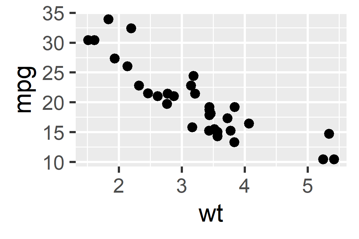
Miles per gallon by weight and horsepower.

Foundations of Data Science

Roadmap

Code Style

Code Style

File Names

Sectioning and Comments

Object Naming

Spacing

Argument Specification

Line Length and Indents

Pipes and Pipelines

Chunk Options

Chunk Options

Hash Pipe Rules

Message

Message

Warning

Error

Eval

Echo

Code Fold

Collapse

Label

Figure Options

Figure Options

Foundations of
Data Science