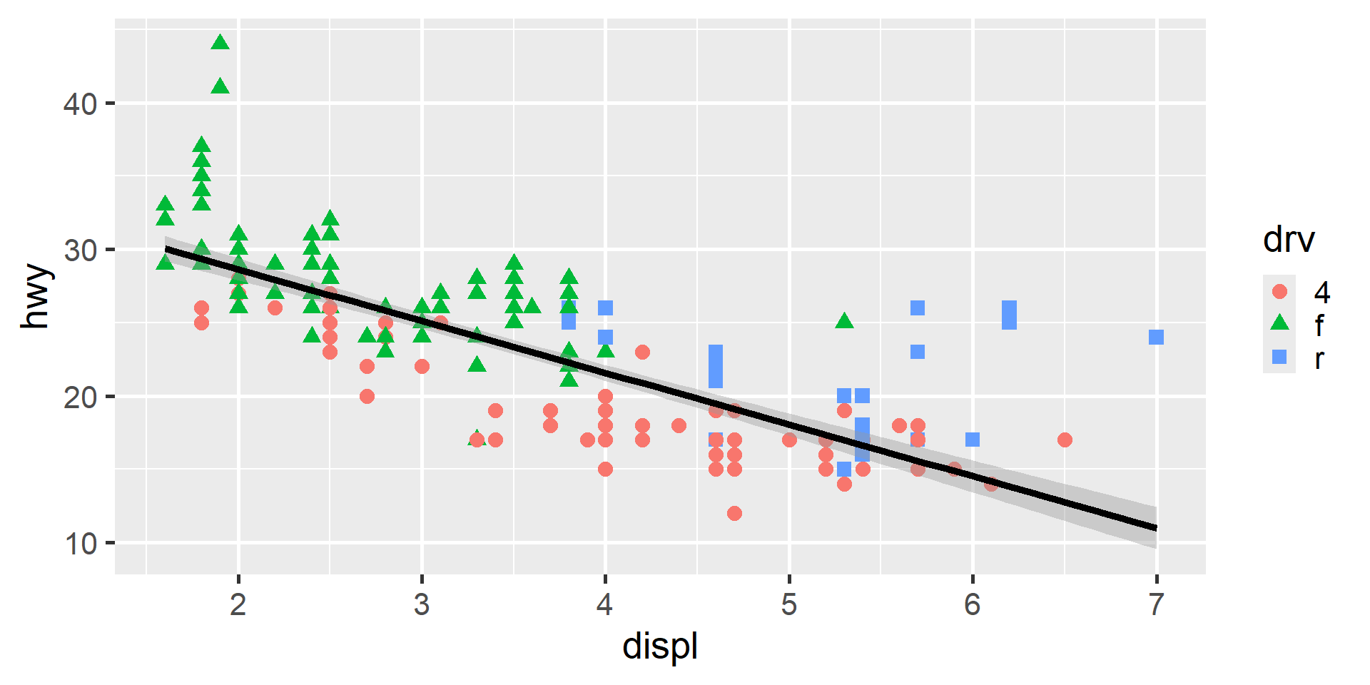
# Create a base plot with default labels and scales
p1 <-
  ggplot(mpg, aes(x = displ, y = hwy)) +
  geom_point(size = 3, aes(color = drv, shape = drv)) +
  geom_smooth(method = "lm", color = "black")
p1Foundations of
Data Science
Spring 2026 | Data 2 (399)
Jeffrey M. Girard | Lecture 06c

Roadmap
- Customize the axis and plot labels in a figure
- Customize the appearance of scales in a figure
Labels
Labels
- By default, scales are named after data variables
- Changing names may enhance communication
- Provide accessible names/definitions
- Include units and other methods info.
- Appear prettier and more professional
- We can also add plot-level information
- Titles and subtitles for take-aways
- Captions for asides or data sources
- This is all done by adding on
labs()
Step 1: The Base Plot
Step 1: The Base Plot
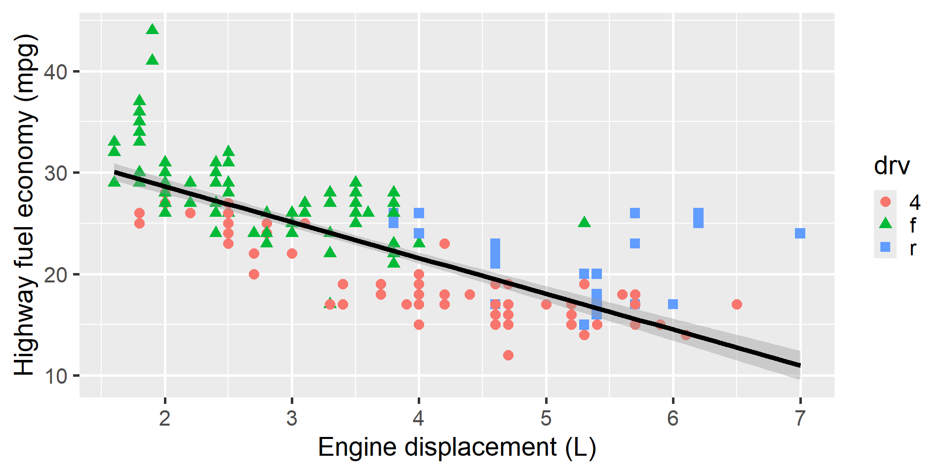
Step 2: Axis Titles
Step 2: Axis Titles
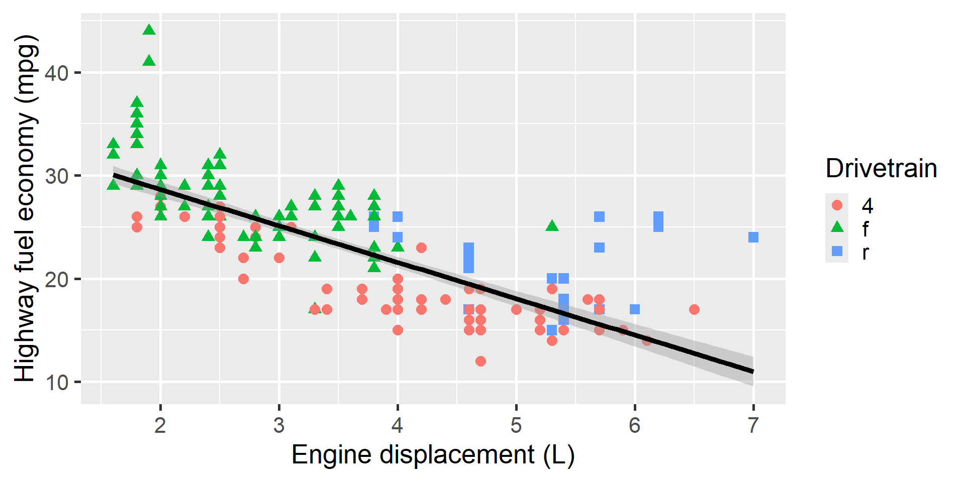
Step 3: Legend Titles
Step 3: Legend Titles
Step 4: Title, Subtitle, and Caption
Step 4: Title, Subtitle, and Caption
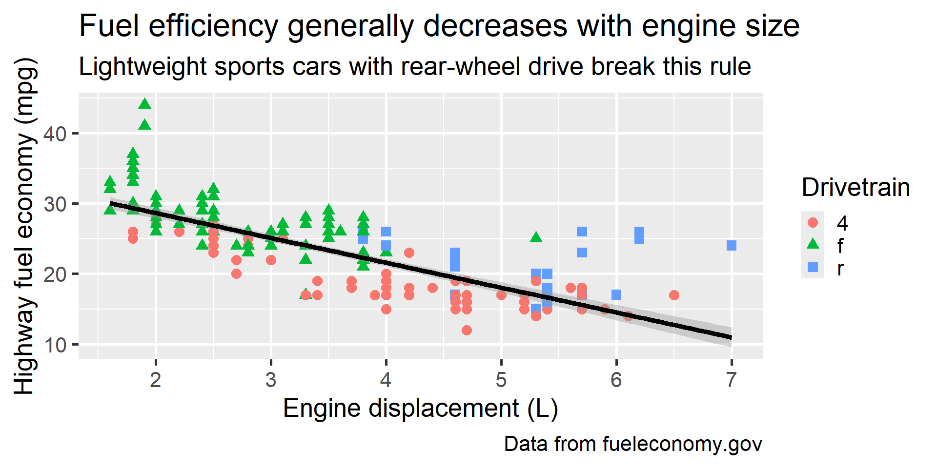
Scales
Scales
- Scales are one of the basic gg elements
- So far, we have let R guess on the scales
- Type (e.g., continuous or discrete)
- Limits (minimum and maximum values)
- Breaks (values to emphasize)
- But we can completely customize the scales!
- Changes may enhance communication
- We will add on various
scale_functions
Step 5: Y-Axis Scale
Step 5: Y-Axis Scale
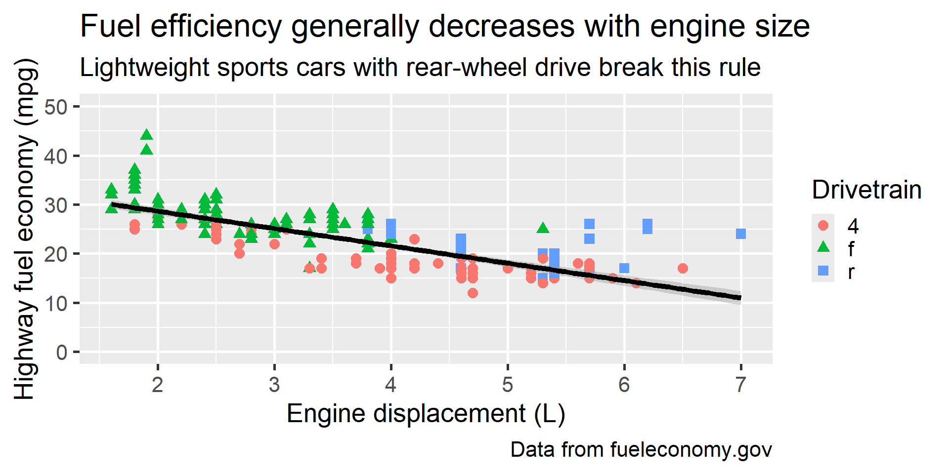
Step 6: X-Axis Scale
Step 6: X-Axis Scale
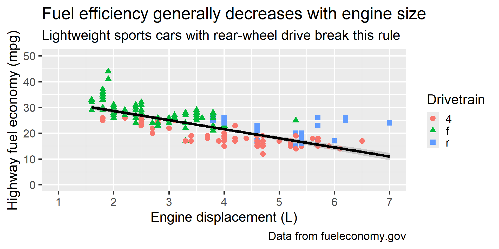
Step 7: Color Scale
Step 7: Color Scale
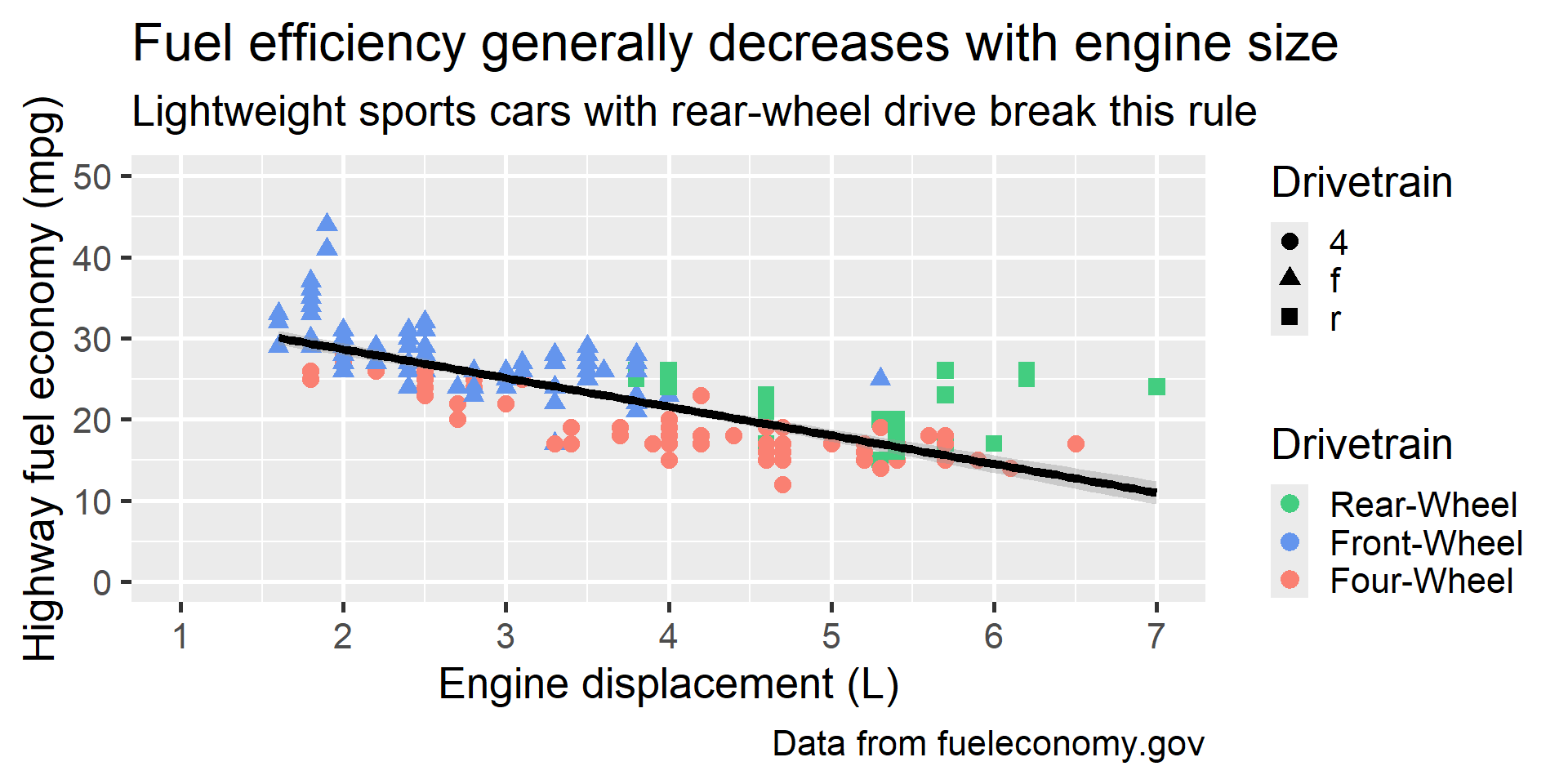
Step 8: Shape Scale
Step 8: Shape Scale
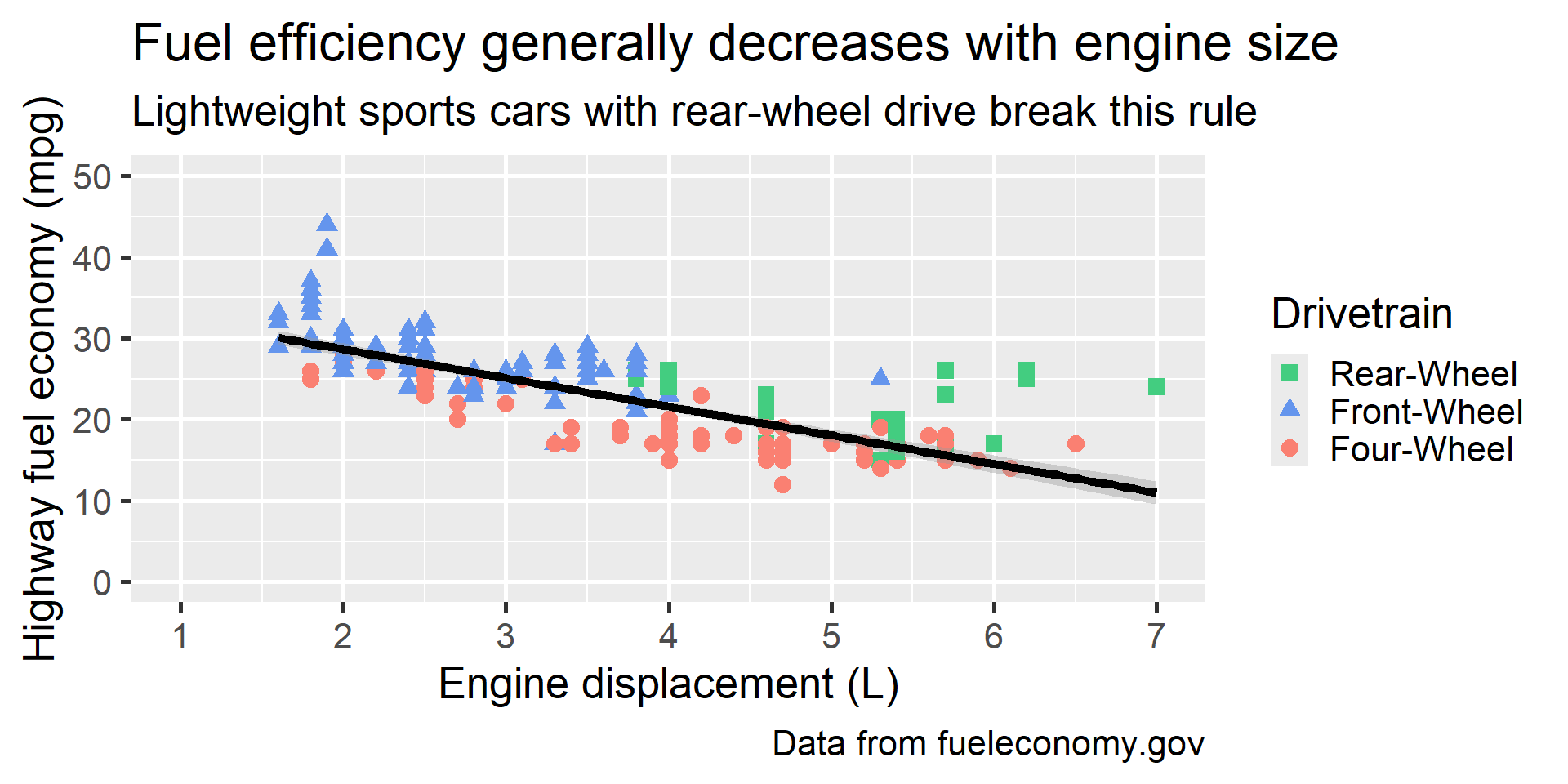
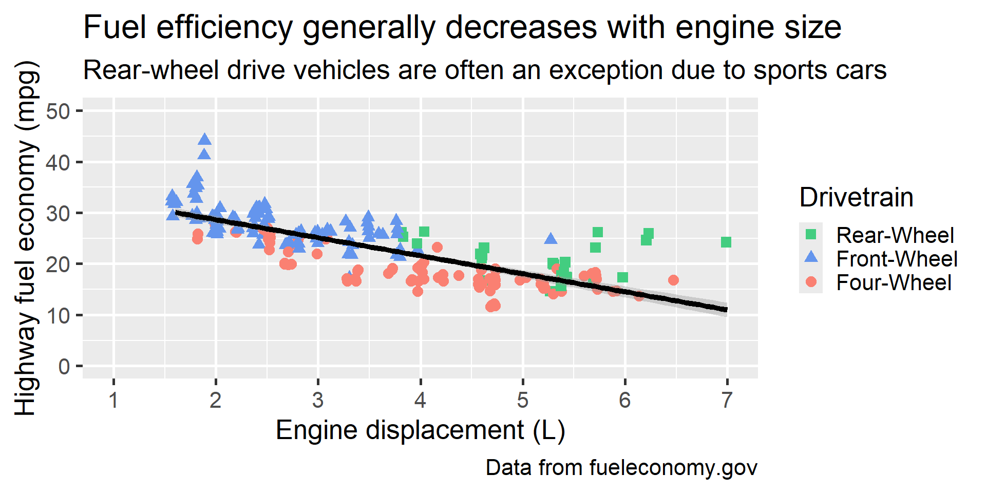
Putting It All Together
ggplot(mpg, aes(x = displ, y = hwy)) +
  geom_jitter(size = 3, aes(color = drv, shape = drv)) +
  geom_smooth(method = "lm", color = "black") +
  labs(
    x = "Engine displacement (L)",
    y = "Highway fuel economy (mpg)",
    color = "Drivetrain",
    shape = "Drivetrain",
    title = "Fuel efficiency generally decreases with engine size",
    subtitle = "Rear-wheel drive vehicles are often an exception due to sports cars",
    caption = "Data from fueleconomy.gov"
  ) +
  scale_y_continuous(
    limits = c(0, 50),
    breaks = seq(0, 50, by = 10)
  ) +
  scale_x_continuous(
    limits = c(1, 7),
    breaks = seq(1, 7, by = 1)
  ) +
  scale_color_manual(
    breaks = c("r", "f", "4"),
    labels = c(
      "4" = "Four-Wheel",
      "f" = "Front-Wheel",
      "r" = "Rear-Wheel"
    ),
    values = c(
      "4" = "salmon",
      "f" = "cornflowerblue",
      "r" = "seagreen3"
    )
  ) +
  scale_shape_discrete(
    breaks = c("r", "f", "4"),
    labels = c(
      "4" = "Four-Wheel",
      "f" = "Front-Wheel",
      "r" = "Rear-Wheel"
    )
  )
Putting It All Together