Foundations of
Data Science

Spring 2026 | Data 2 (399)
Jeffrey M. Girard | Lecture 10a

Roadmap

Understand the difference between samples and populations
Learn the structure of independent and dependent groups
Run group comparisons using afex and easystats

EDA vs. Inference

The Trap of the Sample

We have been turning data into tables and figures
- This is called Exploratory Data Analysis (EDA)

This only tells us about our specific data
- These tables and figures don’t tell us whether the patterns we saw are universally true

We often want to generalize beyond our data
- If Group A has a higher mean than Group B in our data, is that also true more broadly?

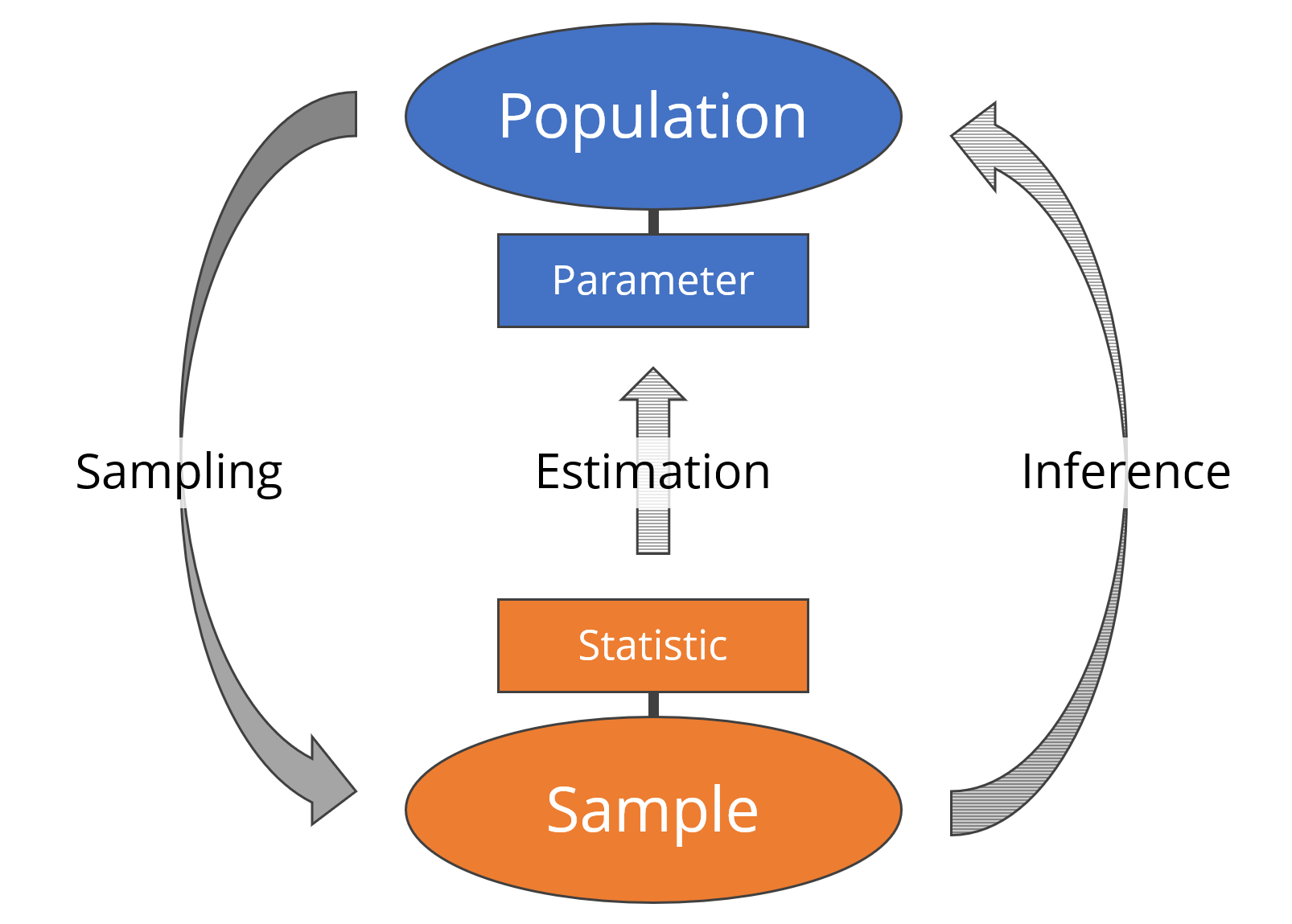
Populations vs. Samples

The Population is the entire group we want to understand
- e.g., All penguins in Antarctica
- We rarely have access to the whole population

The Sample is the subset of data we actually collected
- e.g., The 344 penguins in our dataset
- Samples are imperfect but may be all we have

Parameters vs. Statistics

A Parameter is the “true” number in the population
- e.g., the real average body mass of all penguins in Antarctica
- This number is fixed, but we usually do not know it

A Statistic is the number we calculate from our sample
- e.g., the average body mass of the penguins we happened to catch
- We use the statistic to estimate the parameter

Sampling Uncertainty is the idea that every sample is different
- If we catch 10 different penguins, our statistic will change slightly
- Statistical tests help us decide if patterns in our sample are “real”

Mapping the Connections

Why Compare Groups?

Comparing groups is a fundamental tool in Data Science. It allows us to move from simply describing data to evaluating impact and making decisions.

Basic Science (Discovery)
- Are there natural differences between categories?
- e.g., Do Adelie penguins differ in body mass from Gentoo penguins?

Applied Science (Intervention)
- Does a specific treatment or change have a real effect?
- e.g., Does a new medication lower blood pressure more than a placebo?

Business & Tech (Optimization)
- Which strategy leads to better outcomes?
- e.g., A/B Testing: Does a red “Buy” button generate more revenue than a blue one?

The Logic of Hypothesis Testing

Every statistical test we will learn uses the same underlying logic

The Null Hypothesis (\(H_0\)): The “baseline” assumption
- It assumes nothing interesting is happening in the population
- For group comparisons, \(H_0\) assumes all group means are exactly equal

The Alternative Hypothesis (\(H_1\)): The “discovery” assumption
- It is the claim about the hypothesis we are looking for evidence to support
- For group comparisons, \(H_1\) assumes at least one group mean is different

The p-value:
- How consistent are our sample data with the Null Hypothesis?
- If p < .05, we (traditionally) begin to doubt \(H_0\) and believe \(H_1\) instead

Group Designs

How is the Data Structured?

Before running any tests, R needs to know how the groups are related.

Independent Groups (Between-Subjects)
- Comparing completely different entities
- e.g., (Male vs. Female) or (Adelie vs. Chinstrap vs. Gentoo) penguins

Dependent Groups (Within-Subjects / Repeated Measures)
- Comparing the exact same entities across different conditions
- e.g., The Same Penguin Chicks on (Day 0 vs. Day 10 vs. Day 20)

Setup: Packages

library(tidyverse) # data prep and visualization
library(afex) # fitting ANOVA statistical models
library(easystats) # extracting info from models
library(marginaleffects) # needed by easystats

The Statistical Engine

The Logic of ANOVA

We will use a statistical model called ANOVA (Analysis of Variance)
- It works for comparing two groups or comparing multiple groups

Conceptually, ANOVA compares signal to noise:
- Signal: How different are the group averages from one another?
- Noise: How much random variation is there within the groups?

If the signal is significantly louder than the noise…
- …we can safely conclude the groups are truly different in the population

Understanding the p-value

When we run our ANOVA, it outputs a p-value (probability value)
- It measures how “surprised” we should be by our sample data if there were actually no real differences in the population

Large p-value (e.g., p = .40): Our data is not surprising. The differences we see could easily just be random sampling noise

Small p-value (e.g., p < .05): Our data is very surprising. It is highly unlikely we would see these differences just by random chance
- We call this statistically significant and conclude the population parameters differ

The Catch: Statistics deals in probabilities, not absolute proofs
- Even with a significant result, there is always a small chance of a “false positive”

Two Independent Groups

1. Preparing the Data

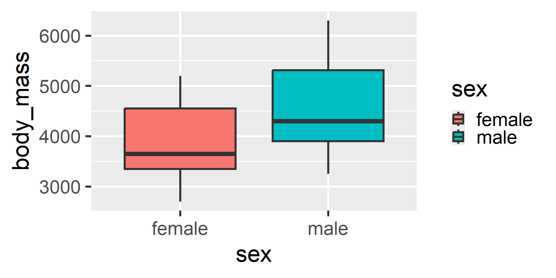
We will use the penguins dataset to compare body mass between Males and Females.

data("penguins", package = "datasets")

dat1 <- 
  penguins |> 
  drop_na(body_mass, sex) |> # Remove penguins with missing data
  mutate(
    id = row_number(), # afex requires an explicit ID column
    sex = factor(sex) # treat sex as a categorical variable
  ) |> 
  select(id, sex, body_mass) # select only used variables

glimpse(dat1)

Rows: 333
Columns: 3
$ id        <int> 1, 2, 3, 4, 5, 6, 7, 8, 9, 10, 11, 12, 13, 14, 15, 16, 17, 1…
$ sex       <fct> male, female, female, female, male, female, male, female, ma…
$ body_mass <int> 3750, 3800, 3250, 3450, 3650, 3625, 4675, 3200, 3800, 4400, …

2. Exploring our Sample

ggplot(dat1, aes(x = sex, y = body_mass, fill = sex)) + geom_boxplot()

3. The Omnibus Test

The aov_ez() function tells us if there are any differences between our groups. Since there are only two groups here, this is mathematically identical to an independent t-test.

fit1 <- aov_ez(
  id = "id",
  dv = "body_mass",
  between = "sex",
  data = dat1
)
model_parameters(fit1)

ANOVA estimation for factorial designs using 'afex'

Parameter | Sum_Squares |  df | Mean_Square |     F |      p
------------------------------------------------------------
sex       |    3.89e+07 |   1 |    3.89e+07 | 72.96 | < .001
Residuals |    1.76e+08 | 331 |    5.33e+05 |       |       

Anova Table (Type 3 tests)

Interpretation: The significant result (p < .001) means the effect of sex is statistically significant. This provides strong evidence to suggest that, in the broader population, the true average body mass differs between male and female penguins.

4. Mean Estimates

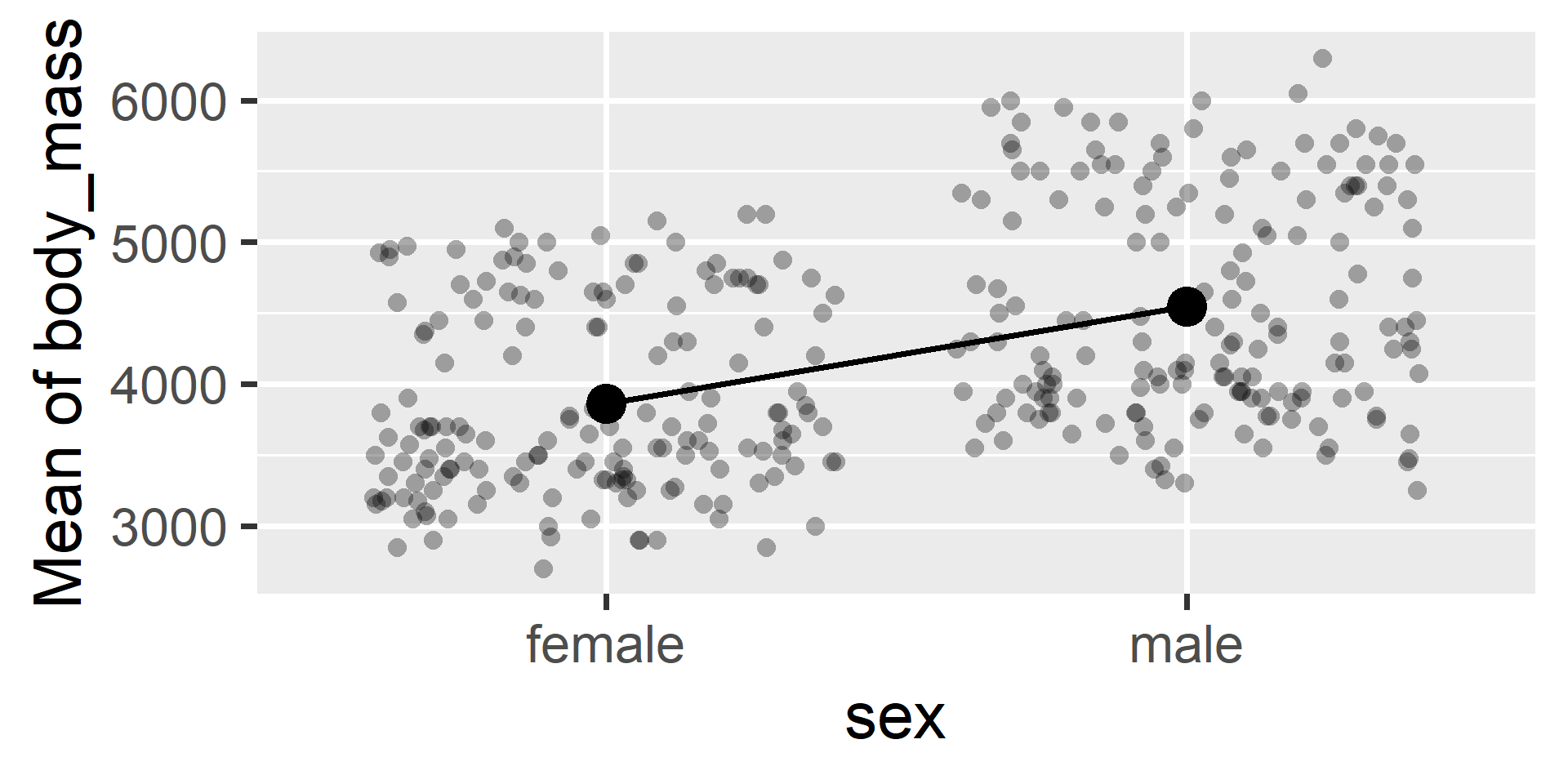
We use estimate_means() to guess what the group means are in the population

We can also plot those model-based estimates (and, optionally, the sample data)

means1 <- estimate_means(fit1) |> print()

Estimated Marginal Means

sex    |    Mean |    SE |             95% CI | t(331)
------------------------------------------------------
female | 3862.27 | 56.83 | [3750.48, 3974.06] |  67.96
male   | 4545.68 | 56.32 | [4434.90, 4656.47] |  80.71

Variable predicted: body_mass
Predictors modulated: sex
Predictors averaged: id

plot(means1, show_data = TRUE)

Three Independent Groups

1. Preparing the Data

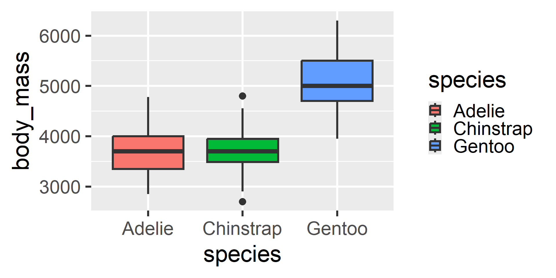
What if we have more than two groups? We use the exact same functions. Let’s start by looking at our penguins data again. We will use the species variable to illustrate this, as there are 3 species represented in this sample.

data("penguins", package = "datasets")

dat2 <- 
  penguins |>
  drop_na(body_mass, species) |> 
  mutate(
    id = row_number(),
    species = factor(species)
  ) |> 
  select(id, species, body_mass)

glimpse(dat2)

Rows: 342
Columns: 3
$ id        <int> 1, 2, 3, 4, 5, 6, 7, 8, 9, 10, 11, 12, 13, 14, 15, 16, 17, 1…
$ species   <fct> Adelie, Adelie, Adelie, Adelie, Adelie, Adelie, Adelie, Adel…
$ body_mass <int> 3750, 3800, 3250, 3450, 3650, 3625, 4675, 3475, 4250, 3300, …

2. Exploring our Sample

ggplot(dat2, aes(x = species, y = body_mass, fill = species)) + geom_boxplot()

3. The Omnibus Test

Now we swap between = "sex" to between = "species".

fit2 <- aov_ez(
  id = "id",
  dv = "body_mass",
  between = "species",
  data = dat2
)
model_parameters(fit2)

ANOVA estimation for factorial designs using 'afex'

Parameter | Sum_Squares |  df | Mean_Square |      F |      p
-------------------------------------------------------------
species   |    1.47e+08 |   2 |    7.34e+07 | 343.63 | < .001
Residuals |    7.24e+07 | 339 |    2.14e+05 |        |       

Anova Table (Type 3 tests)

Interpretation: The significant result (p < .001) suggests that the true average body mass in the population is not identical across all three species. This gives us evidence that species is related to mass, though we cannot yet say which specific ones differ.

4. Estimating Means

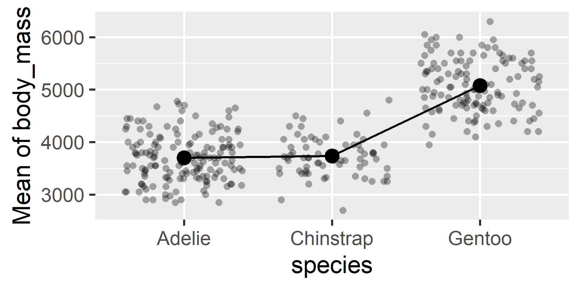
means2 <- estimate_means(fit2) |> print()

Estimated Marginal Means

species   |    Mean |    SE |             95% CI | t(339)
---------------------------------------------------------
Adelie    | 3700.66 | 37.62 | [3626.67, 3774.66] |  98.37
Chinstrap | 3733.09 | 56.06 | [3622.82, 3843.36] |  66.59
Gentoo    | 5076.02 | 41.68 | [4994.03, 5158.00] | 121.78

Variable predicted: body_mass
Predictors modulated: species
Predictors averaged: id

plot(means2, show_data = TRUE)

5. Contrasting Groups

The estimate_contrasts() function automatically tests all pairs and adjusts the p-values to protect us from false positives (due to multiple tests).

estimate_contrasts(fit2, p_adjust = "holm")

Marginal Contrasts Analysis

Level1    | Level2    | Difference |    SE |             95% CI | t(339) |      p
---------------------------------------------------------------------------------
Chinstrap | Adelie    |      32.43 | 67.51 | [-100.37,  165.22] |   0.48 |  0.631
Gentoo    | Adelie    |    1375.35 | 56.15 | [1264.91, 1485.80] |  24.50 | < .001
Gentoo    | Chinstrap |    1342.93 | 69.86 | [1205.52, 1480.34] |  19.22 | < .001

Variable predicted: body_mass
Predictors contrasted: species
Predictors averaged: id
p-value adjustment method: Holm (1979)

Interpretation: We found significant differences (p < .001) when comparing Gentoos to both Adelies and Chinstraps, suggesting these mass differences likely exist in the population. However, the difference between Chinstraps and Adelies was not significant (p > .05), meaning we lack evidence to say their true population means differ.

Three Dependent Groups

1. Preparing the Data

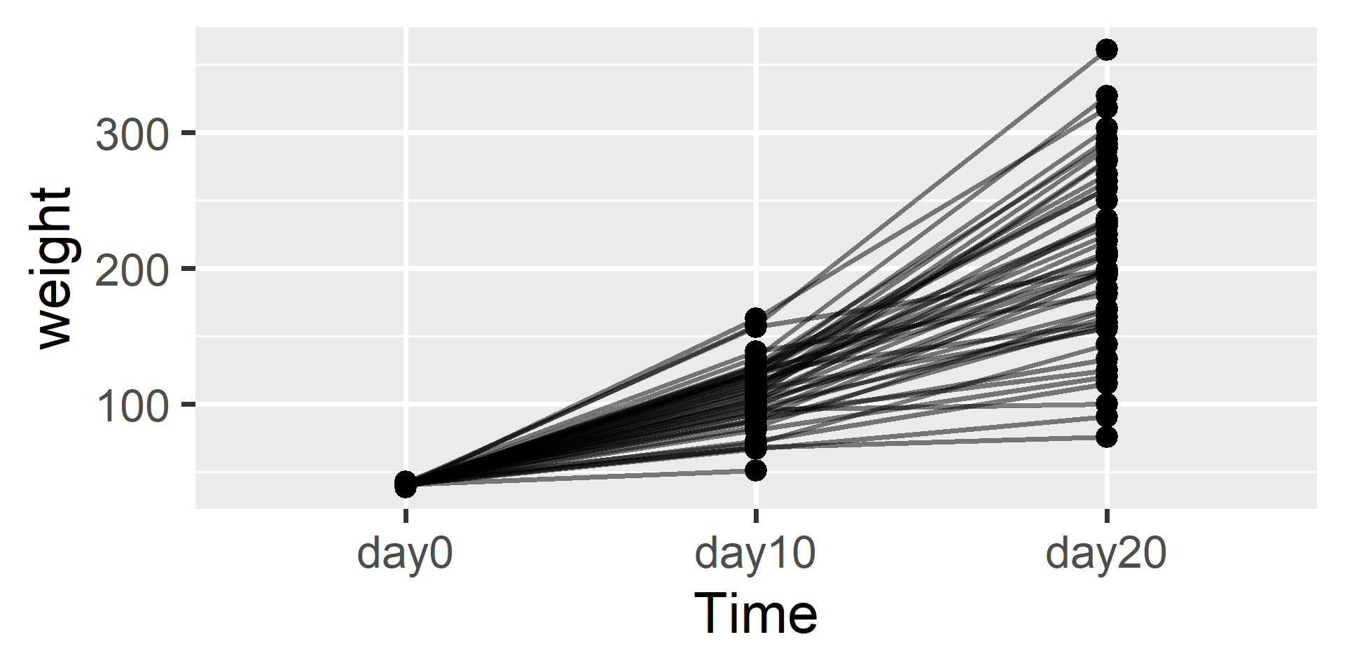
When testing the same subjects multiple times, the data must be in a long format. We will use the ChickWeight dataset to see if chicks gained weight between Days 0, 10, and 20.

data("ChickWeight", package = "datasets")

dat3 <- 
  ChickWeight |>
  drop_na(weight, Time) |> 
  filter(Time %in% c(0, 10, 20)) |>
  mutate(Time = factor(Time, labels = c("day0", "day10", "day20"))) |> 
  select(Chick, Time, weight)

glimpse(dat3)

Rows: 145
Columns: 3
$ Chick  <ord> 1, 1, 1, 2, 2, 2, 3, 3, 3, 4, 4, 4, 5, 5, 5, 6, 6, 6, 7, 7, 7, …
$ Time   <fct> day0, day10, day20, day0, day10, day20, day0, day10, day20, day…
$ weight <dbl> 42, 93, 199, 40, 103, 209, 43, 99, 198, 42, 87, 160, 41, 106, 2…

2. Exploring our Sample

ggplot(dat3, aes(x = Time, y = weight, group = Chick)) + 
  geom_point() + 
  geom_line(alpha = 0.5)

3. The Omnibus Test

To tell R to run a dependent test, swap the between argument for within

fit3 <- aov_ez(
  id = "Chick", 
  dv = "weight",
  within = "Time", 
  data = dat3
)
model_parameters(fit3)

ANOVA estimation for factorial designs using 'afex'

Parameter | Sum_Squares | Sum_Squares_Error |   df | df (error) | Mean_Square |      F |      p
-----------------------------------------------------------------------------------------------
Time      |    6.62e+05 |          1.16e+05 | 1.11 |      50.13 |     2306.78 | 257.45 | < .001

Anova Table (Type 3 tests)

Interpretation: The significant p-value (p < .001) indicates that the true average weight of the population likely does not stay constant across these three time points. This points to a broader growth trend beyond just our specific sample.

4. Estimating Means

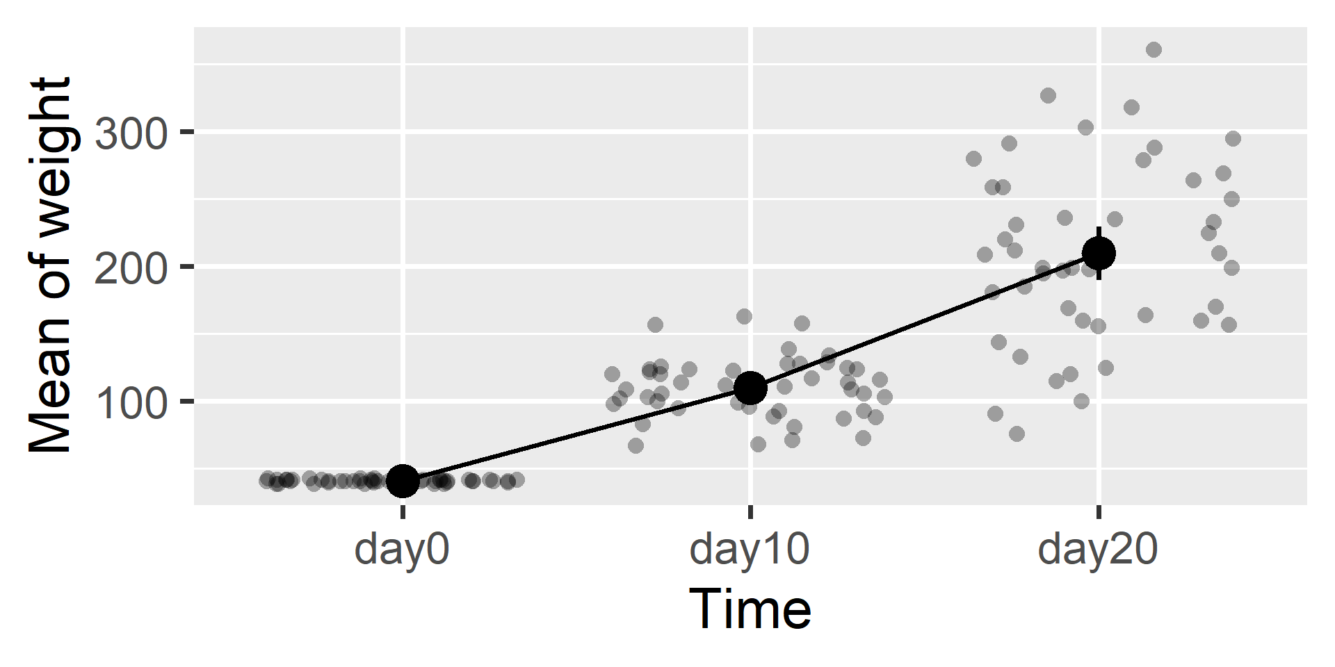
means3 <- estimate_means(fit3) |> print()

Estimated Marginal Means

Time  |   Mean |   SE |           95% CI |  t(45)
-------------------------------------------------
day0  |  41.09 | 0.17 | [ 40.75,  41.42] | 246.20
day10 | 109.72 | 3.30 | [103.07, 116.36] |  33.25
day20 | 209.72 | 9.81 | [189.97, 229.47] |  21.39

Variable predicted: weight
Predictors modulated: Time
Predictors averaged: Chick

plot(means3, show_data = TRUE)

5. Contrasting Groups

estimate_contrasts(fit3, p_adjust = "holm")

Marginal Contrasts Analysis

Level1 | Level2 | Difference |   SE |           95% CI | t(45) |      p
-----------------------------------------------------------------------
day10  | day0   |      68.63 | 3.34 | [ 61.91,  75.36] | 20.56 | < .001
day20  | day0   |     168.63 | 9.86 | [148.77, 188.49] | 17.10 | < .001
day20  | day10  |     100.00 | 7.69 | [ 84.50, 115.50] | 13.00 | < .001

Variable predicted: weight
Predictors contrasted: Time
Predictors averaged: Chick
p-value adjustment method: Holm (1979)

Interpretation: All three pairwise comparisons are statistically significant. This provides evidence to suggest that the true average weight in the population increases at each of these measured intervals (from Day 0 to 10, and Day 10 to 20).

Foundations of Data Science

Roadmap

EDA vs. Inference

The Trap of the Sample

Populations vs. Samples

Parameters vs. Statistics

Mapping the Connections

Why Compare Groups?

The Logic of Hypothesis Testing

Group Designs

How is the Data Structured?

Setup: Packages

The Statistical Engine

The Logic of ANOVA

Understanding the p-value

Two Independent Groups

1. Preparing the Data

2. Exploring our Sample

3. The Omnibus Test

4. Mean Estimates

Three Independent Groups

1. Preparing the Data

2. Exploring our Sample

3. The Omnibus Test

4. Estimating Means

5. Contrasting Groups

Three Dependent Groups

1. Preparing the Data

2. Exploring our Sample

3. The Omnibus Test

4. Estimating Means

5. Contrasting Groups

Foundations of
Data Science