Foundations of
Data Science

Spring 2026 | Data 2 (399)
Jeffrey M. Girard | Lecture 10b

Roadmap

  • Run correlation tests for continuous variables

  • Run Chi-Square tests for categorical variables

Moving Beyond Groups

Last lecture, we compared a continuous variable across different categories

  • What if we want to test the association of two continuous variables?
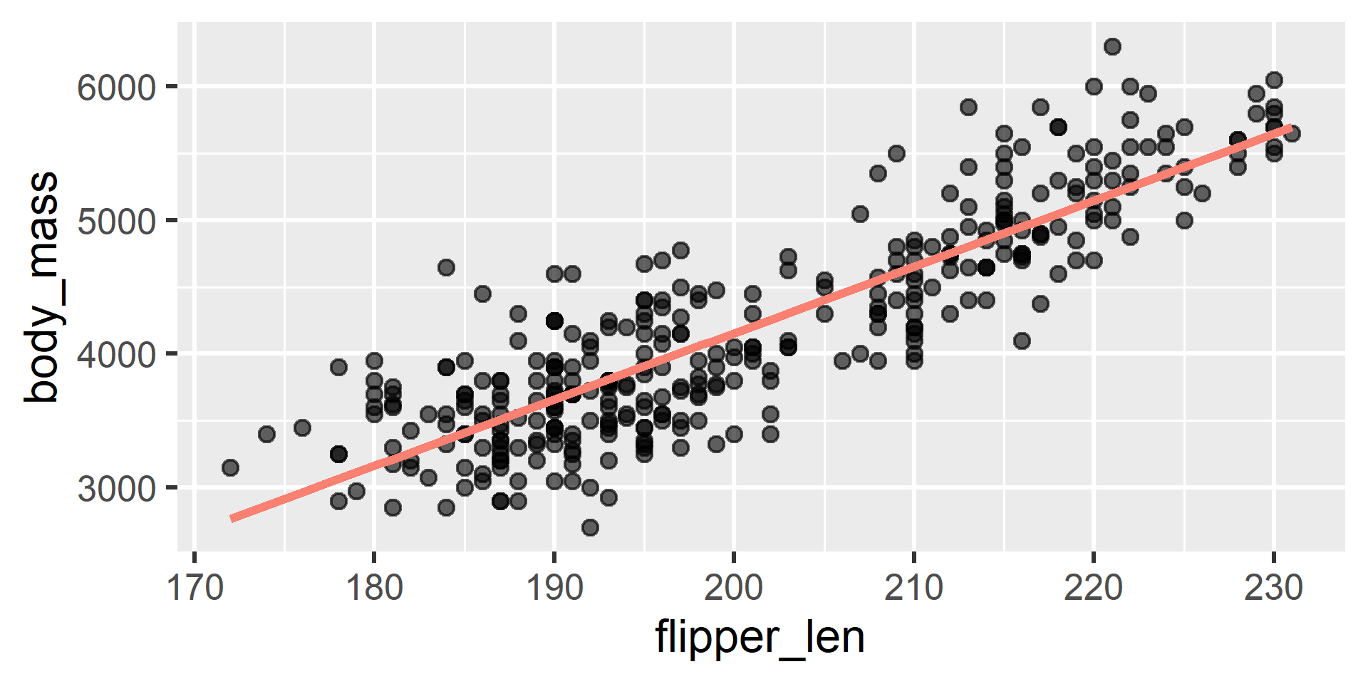
    • e.g., As a penguin’s flipper gets longer, does its body mass also increase?
    • We can use Correlation to test this
  • What if we want to test the association of two categorical variables?
    • e.g., Does the species of a penguin depend on which island it lives on?
    • We can use Chi-Square to test this

Correlations

Interpreting Correlations

  • A correlation (parameter = \(\rho\), statistic = \(r\)) quantifies the direction and strength of the linear relationship between two variables (how closely the points form a straight line)

  • Hypotheses:

    • \(H_0\): \(\rho = 0\) (There is no linear relationship in the population)
    • \(H_1\): \(\rho \neq 0\) (There is a linear relationship in the population)
  • Direction: do the variables change together or opposing?

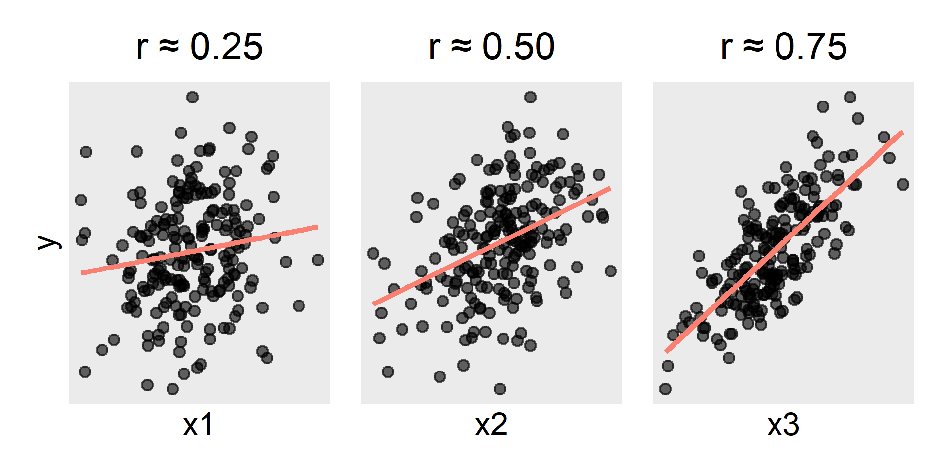
    • \(r > 0\): the variables change together
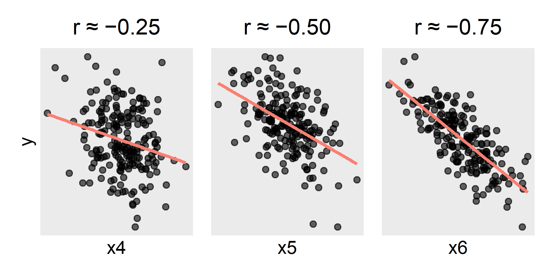
    • \(r < 0\): the variables change in opposition
  • Strength: how well does one variable predict the other?

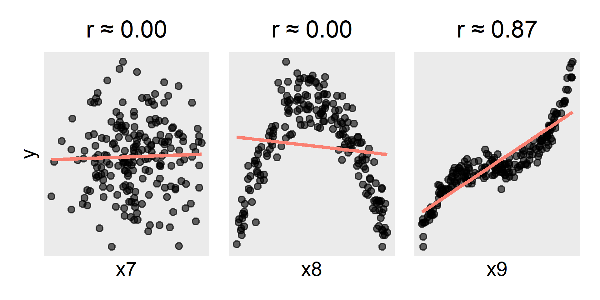
    • \(r \to 0\): no linear relationship (but maybe a non-linear one)
    • \(r \to \pm 1\): perfect (positive or negative) linear relationship

Positive linear

Negative linear

No linear / Nonlinear

1. Preparing the Data

library(tidyverse)
library(easystats)

data("penguins", package = "datasets")

dat1 <- penguins |> select(flipper_len, body_mass)

glimpse(dat1)
Rows: 344
Columns: 2
$ flipper_len <int> 181, 186, 195, NA, 193, 190, 181, 195, 193, 190, 186, 180,…
$ body_mass   <int> 3750, 3800, 3250, NA, 3450, 3650, 3625, 4675, 3475, 4250, …
2. Exploring our Sample

ggplot(dat1, aes(x = flipper_len, y = body_mass)) + 
  geom_point(alpha = 0.6) +
  geom_smooth(method = "lm", se = FALSE, color = "salmon")

3. The Correlation Test

res1 <- correlation(dat1) |> print()
# Correlation Matrix (pearson-method)

Parameter1  | Parameter2 |    r |       95% CI | t(340) |         p
-------------------------------------------------------------------
flipper_len |  body_mass | 0.87 | [0.84, 0.89] |  32.72 | < .001***

p-value adjustment method: Holm (1979)
Observations: 342

Interpretation: The correlation (\(r\)) is 0.87. The significant result (p < .001) provides evidence that flipper length and body mass are positively associated in the population: penguins with more (or less) body mass tend to have longer (or shorter) flippers.

4. Multiple Variables

dat2 <- 
  penguins |> 
  select(bill_len, bill_dep, flipper_len, body_mass)

res2 <- correlation(dat2, p_adjust = "holm") |> print()
# Correlation Matrix (pearson-method)

Parameter1  |  Parameter2 |     r |         95% CI | t(340) |         p
-----------------------------------------------------------------------
bill_len    |    bill_dep | -0.24 | [-0.33, -0.13] |  -4.46 | < .001***
bill_len    | flipper_len |  0.66 | [ 0.59,  0.71] |  16.03 | < .001***
bill_len    |   body_mass |  0.60 | [ 0.52,  0.66] |  13.65 | < .001***
bill_dep    | flipper_len | -0.58 | [-0.65, -0.51] | -13.26 | < .001***
bill_dep    |   body_mass | -0.47 | [-0.55, -0.39] |  -9.87 | < .001***
flipper_len |   body_mass |  0.87 | [ 0.84,  0.89] |  32.72 | < .001***

p-value adjustment method: Holm (1979)
Observations: 342

4. The Correlation Matrix

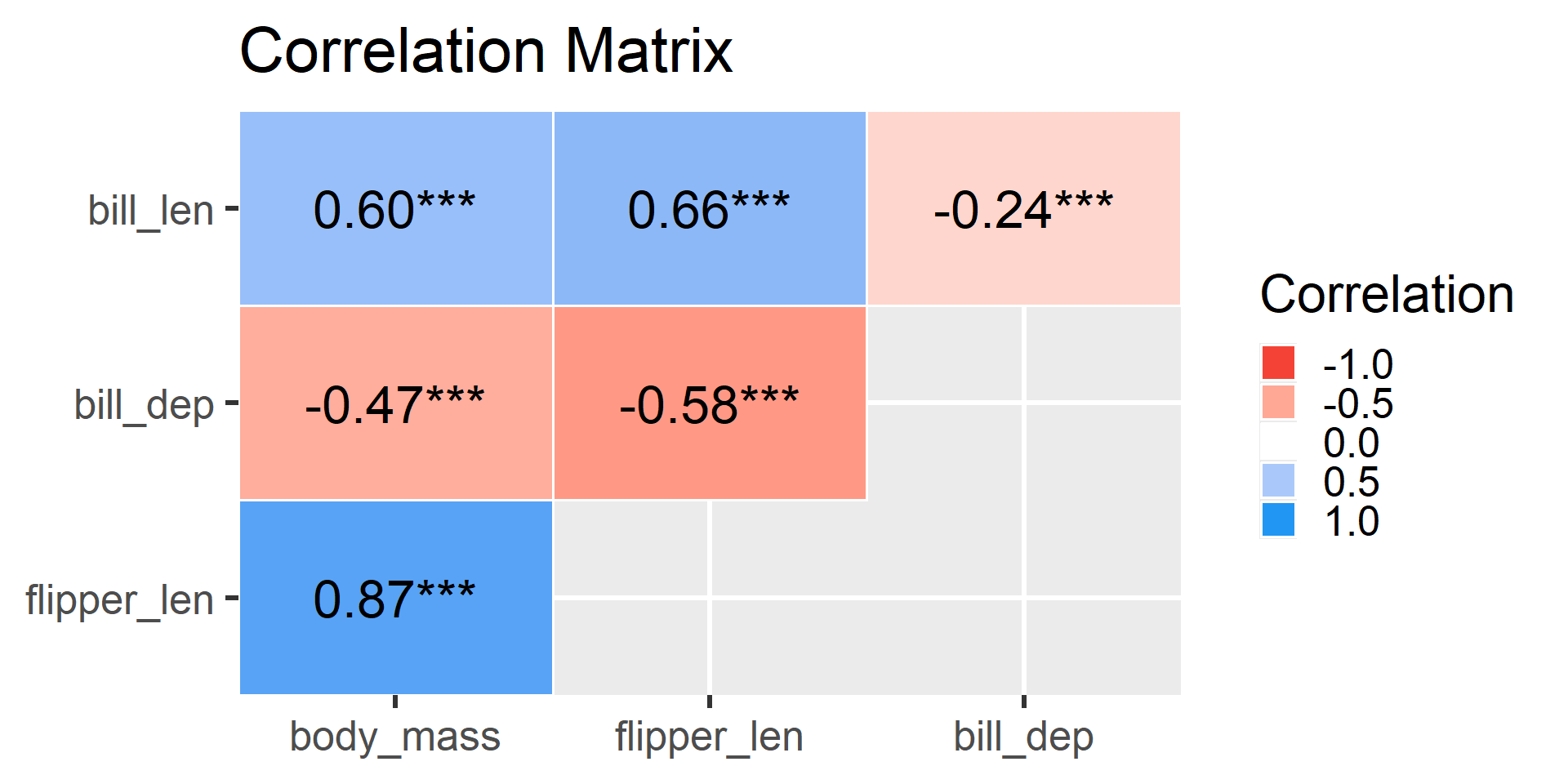
mat2 <- summary(res2) |> print()
# Correlation Matrix (pearson-method)

Parameter   | body_mass | flipper_len | bill_dep
------------------------------------------------
bill_len    |   0.60*** |     0.66*** | -0.24***
bill_dep    |  -0.47*** |    -0.58*** |         
flipper_len |   0.87*** |             |         

p-value adjustment method: Holm (1979)

Interpretation: The function automatically tests every possible pair of variables and provides adjusted \(p\)-values for each relationship.

5. Visualizing the Matrix

plot(mat2)

Two Categorical Variables

Understanding Chi-Square

The Chi-Square \((\chi^2)\) Test of Independence looks at categorical relationships

  • The Core Question:
    • Does knowing one category tell us something about the other category?
    • e.g., Are the Species and Island categorical variables associated?
  • The Hypotheses:
    • Null Hypothesis (\(H_0\)): The variables are completely independent
      • e.g., species are randomly distributed across islands
    • Alternative Hypothesis (\(H_1\)): The variables are associated
      • e.g., some species are more common on some islands
  • We look at frequencies (counts) of each combination of categories

1. Preparing the Data

data("penguins", package = "datasets")

dat3 <- penguins |> select(species, island)

glimpse(dat3)
Rows: 344
Columns: 2
$ species <fct> Adelie, Adelie, Adelie, Adelie, Adelie, Adelie, Adelie, Adelie…
$ island  <fct> Torgersen, Torgersen, Torgersen, Torgersen, Torgersen, Torgers…

2. Exploring our Sample

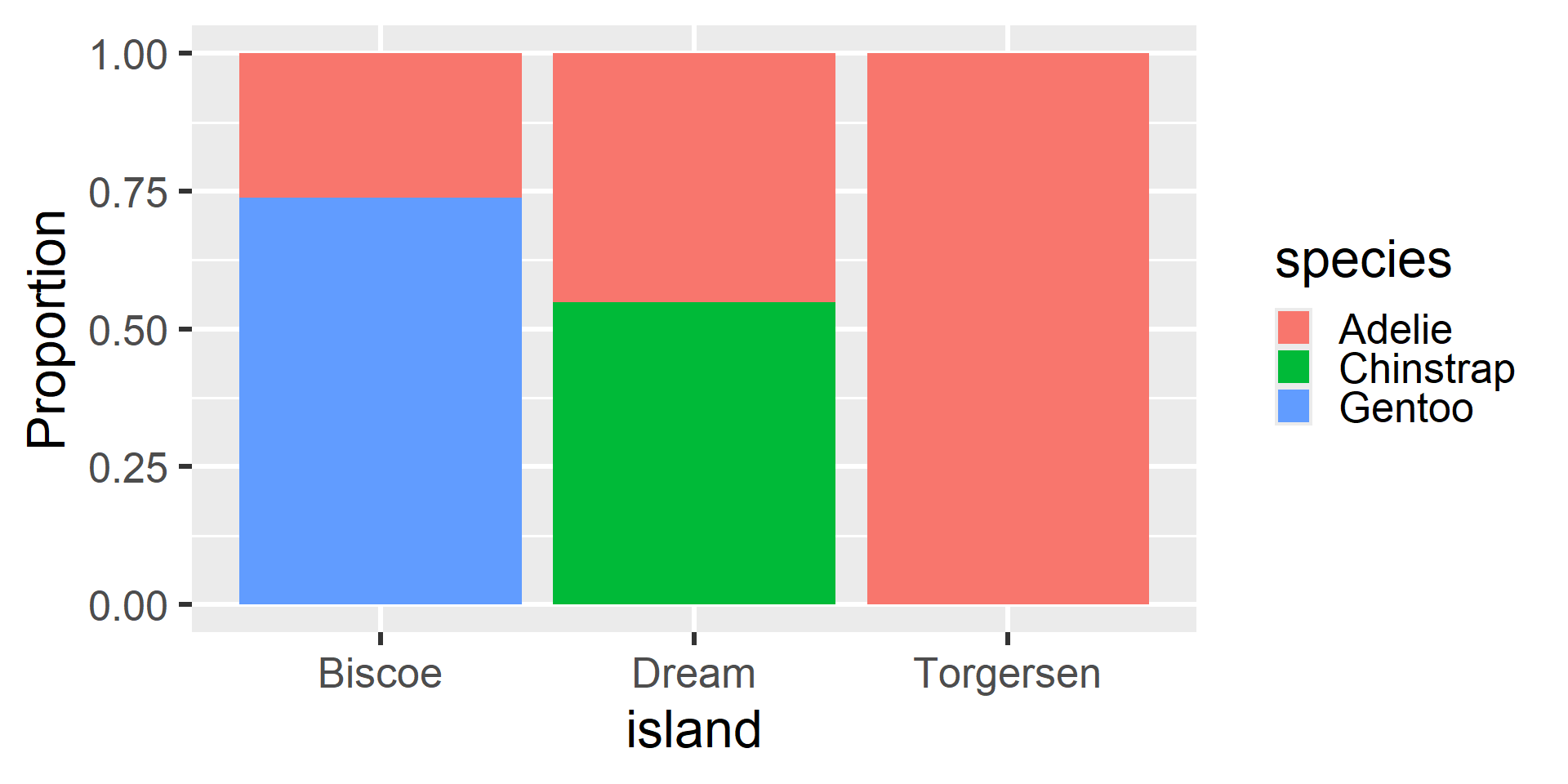
ggplot(dat3, aes(x = island, fill = species)) + 
  geom_bar(position = "fill") + # "fill" makes all bars the same height
  labs(y = "Proportion")

3. Cross-Tabulation

Before we can test these variables, we need to count how many penguins fall into each combination of categories. We use the xtabs() function for this

The syntax uses a one-sided formula ~ variable1 + variable2

tab3 <- dat3 |> table() |> print()
           island
species     Biscoe Dream Torgersen
  Adelie        44    56        52
  Chinstrap      0    68         0
  Gentoo       124     0         0

Note: All Gentoo penguins were observed on Biscoe, and all Chinstrap penguins were observed on Dream This suggests a very strong association!

4. The Logic of Chi-Square

How does a Chi-Square test actually work?

  • It compares what we observed in our data to what we would expect to see if the two variables were completely independent.
  • If species and island were unrelated, penguins would be distributed across the islands purely based on the overall size of each island and the overall population of each species.
  • The larger the difference between Observed and Expected, the larger our resulting Chi-Square statistic (\(\chi^2\)).
res3 <- chisq.test(tab3)

5. Expected Frequencies

R can calculate those “Expected” numbers for us, and we can compare them

res3$observed
           island
species     Biscoe Dream Torgersen
  Adelie        44    56        52
  Chinstrap      0    68         0
  Gentoo       124     0         0
res3$expected
           island
species       Biscoe    Dream Torgersen
  Adelie    74.23256 54.79070  22.97674
  Chinstrap 33.20930 24.51163  10.27907
  Gentoo    60.55814 44.69767  18.74419

Note: These tables are very different! If there were no association, we would expect to find about 45 Gentoo on Dream. But in our sample, we found 0

6. The Chi-Square Test

Now we look at the formal test results using model_parameters()

model_parameters(res3)
Pearson's Chi-squared test

Chi2(4) |      p
----------------
299.55  | < .001

Interpretation: The highly significant result (p < .001) means the distribution of species is dependent on the island. We have strong evidence that this geographic sorting exists in the broader population.

Wrap-Up

Choosing the Right Test

You now have three primary tools for testing basic bivariate relationships

Variable 1 Variable 2 Test R Function
Categorical Continuous ANOVA aov_ez()
Continuous Continuous Correlation correlation()
Categorical Categorical Chi-Square chisq.test()


Note: “Bivariate” means we are only looking at two variables at a time.
In future courses, you will learn how to build models with many variables!