Foundations of
Data Science

Spring 2026 | Data 2 (399)
Jeffrey M. Girard | Lecture 11b

Roadmap

Identify when “wide” or “long” format is needed
Reshape wide data into long data using pivot_longer()
Reshape long data into wide data using pivot_wider()

Pivot Longer

Tidy data can have many different shapes.
- Long format is useful for group summaries and most plots.
- Wide format is useful for correlations and calculating differences.

pivot_longer() adds rows from columns.
- cols: select the columns we want to pivot.
- names_to: create a new column where the old names will go (provide as a “string”).
- values_to: create a new column where the old values will go (provide as a “string”).

Preparing the Data

First, let’s simulate a dataset in wide format.

gradebook <- tibble(
  student = 1:10,
  test1 = round(rnorm(n = 10, mean = 77, sd = 9)),
  test2 = round(rnorm(n = 10, mean = 75, sd = 8)),
  test3 = round(rnorm(n = 10, mean = 80, sd = 7))
)
gradebook

# A tibble: 10 × 4
  student test1 test2 test3
    <int> <dbl> <dbl> <dbl>
1       1    66    71    81
2       2    79    67    77
3       3    87    69    77
4       4    56    76    83
5       5    81    83    75
6       6    82    74    70
# ℹ 4 more rows

The Problem with Wide Data

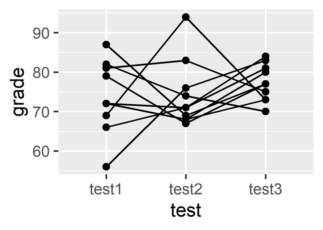
Question: How do we plot the trend of grades across tests for each student?

glimpse(gradebook)

Rows: 10
Columns: 4
$ student <int> 1, 2, 3, 4, 5, 6, 7, 8, 9, 10
$ test1   <dbl> 66, 79, 87, 56, 81, 82, 72, 72, 72, 69
$ test2   <dbl> 71, 67, 69, 76, 83, 74, 71, 68, 68, 94
$ test3   <dbl> 81, 77, 77, 83, 75, 70, 84, 73, 80, 73

# We cannot map test and grade to x and y because they aren't columns!
ggplot(gradebook, aes(x = ???, y = ???, group = student)) + ...

# What we need are test and grade columns
ggplot(gradebook, aes(x = test, y = grade, group = student)) + ...

Basic pivot_longer()

gradebook2 <- gradebook |> 
  pivot_longer(
    cols = c(test1, test2, test3), 
    names_to = "test", 
    values_to = "grade"
  ) 
gradebook2

# A tibble: 30 × 3
  student test  grade
    <int> <chr> <dbl>
1       1 test1    66
2       1 test2    71
3       1 test3    81
4       2 test1    79
5       2 test2    67
6       2 test3    77
# ℹ 24 more rows

Plotting Long Data

Now that we have the data in long format, plotting is easy!

ggplot(
  gradebook2, 
  aes(
    x = test, 
    y = grade, 
    group = student
  )
) + 
  geom_line() + 
  geom_point()

Convenience Options

gradebook |> 
  pivot_longer(
    cols = starts_with("test"), # tidy select cols
    names_to = "test", 
    values_to = "grade",
    names_prefix = "test", # remove prefix from names
    names_transform = parse_number # turn names into numbers
  )

# A tibble: 30 × 3
  student  test grade
    <int> <dbl> <dbl>
1       1     1    66
2       1     2    71
3       1     3    81
4       2     1    79
5       2     2    67
6       2     3    77
# ℹ 24 more rows

Numeric Column Names

Datasets with numeric columns names can cause issues…

data("table4a", package = "tidyr")
table4a

# A tibble: 3 × 3
  country     `1999` `2000`
  <chr>        <dbl>  <dbl>
1 Afghanistan    745   2666
2 Brazil       37737  80488
3 China       212258 213766

table4a |> select(1999, 2000)

Error in `select()`:
! Can't select columns past the end.
ℹ Locations 1999 and 2000 don't exist.
ℹ There are only 3 columns.

table4a |> select(`1999`, `2000`)

# A tibble: 3 × 2
  `1999` `2000`
   <dbl>  <dbl>
1    745   2666
2  37737  80488
3 212258 213766

Pivoting Such Columns

table4a |> 
  pivot_longer(
    cols = c(`1999`, `2000`),
    names_to = "year",
    values_to = "cases"
  )

# A tibble: 6 × 3
  country     year   cases
  <chr>       <chr>  <dbl>
1 Afghanistan 1999     745
2 Afghanistan 2000    2666
3 Brazil      1999   37737
4 Brazil      2000   80488
5 China       1999  212258
6 China       2000  213766

Pivot Wider

Tidy data can have many different shapes.
- Long format is useful for group summaries and most plots.
- Wide format is useful for correlations and calculating differences.

pivot_wider() adds columns from rows.
- names_from: select the columns containing the new column names.
- values_from: select the columns containing the data values.

Preparing the Data

First, let’s simulate a dataset in long format.

diary_data <- tibble(
    participant = rep(1:3, each = 7, times = 2),
    day = rep(1:7, each = 2, times = 3),
    scale = rep(c("mood", "sleep"), times = 3*7),
    score = round(rnorm(n = 3*7*2), digits = 1)
  )
diary_data

# A tibble: 42 × 4
  participant   day scale score
        <int> <int> <chr> <dbl>
1           1     1 mood    1.1
2           1     1 sleep  -0.5
3           1     2 mood   -0.7
4           1     2 sleep  -0.5
5           1     3 mood   -1.6
6           1     3 sleep  -1.2
# ℹ 36 more rows

The Problem with Long Data

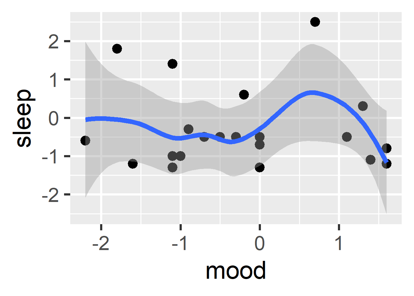
Question: Does daily mood correlate with daily sleep?

glimpse(diary_data)

Rows: 42
Columns: 4
$ participant <int> 1, 1, 1, 1, 1, 1, 1, 2, 2, 2, 2, 2, 2, 2, 3, 3, 3, 3, 3, 3…
$ day         <int> 1, 1, 2, 2, 3, 3, 4, 4, 5, 5, 6, 6, 7, 7, 1, 1, 2, 2, 3, 3…
$ scale       <chr> "mood", "sleep", "mood", "sleep", "mood", "sleep", "mood",…
$ score       <dbl> 1.1, -0.5, -0.7, -0.5, -1.6, -1.2, -2.2, -1.3, -0.3, -0.5,…

# We cannot map mood and sleep to x and y because they aren't columns!
ggplot(diary_data, aes(x = ???, y = ???)) + ...

# What we need are mood and sleep columns
ggplot(diary_data, aes(x = mood, y = sleep)) + ...

Basic pivot_wider()

diary_data |>
  pivot_wider(
    names_from = scale,
    values_from = score
  )

# A tibble: 21 × 4
  participant   day  mood sleep
        <int> <int> <dbl> <dbl>
1           1     1   1.1  -0.5
2           1     2  -0.7  -0.5
3           1     3  -1.6  -1.2
4           1     4  -2.2  -0.6
5           2     4   0    -1.3
6           2     5  -0.3  -0.5
# ℹ 15 more rows

Plotting Wide Data

Now that we have the data in wide format, plotting is easy!

diary_data |> 
  pivot_wider(
    names_from = scale,
    values_from = score
  ) |> 
  ggplot(aes(x = mood, y = sleep)) + 
  geom_point() +
  geom_smooth()

Numerical Column Names

Sometimes pivoting leaves you with column names that are just numbers.

diary_data |> 
  pivot_wider(
    names_from = day,
    values_from = score
  )

# A tibble: 6 × 9
  participant scale   `1`   `2`   `3`   `4`   `5`   `6`   `7`
        <int> <chr> <dbl> <dbl> <dbl> <dbl> <dbl> <dbl> <dbl>
1           1 mood    1.1  -0.7  -1.6  -2.2  -1.1  -0.2   1.6
2           1 sleep  -0.5  -0.5  -1.2  -0.6  -1     0.6  -0.8
3           2 sleep  -1.2   2.5  -0.7  -1.3  -0.5  -1.1  -0.3
4           2 mood    1.6   0.7   0     0    -0.3   1.4  -0.9
5           3 mood   -1    -1.1  -0.5  -1.8  -1.1   1.3   0  
6           3 sleep  -1    -1.3  -0.5   1.8   1.4   0.3  -0.5

Avoiding Such Columns

We can use names_prefix to make them clearer and easier to work with.

diary_data |> 
  pivot_wider(
    names_from = day,
    values_from = score,
    names_prefix = "day_"
  )

# A tibble: 6 × 9
  participant scale day_1 day_2 day_3 day_4 day_5 day_6 day_7
        <int> <chr> <dbl> <dbl> <dbl> <dbl> <dbl> <dbl> <dbl>
1           1 mood    1.1  -0.7  -1.6  -2.2  -1.1  -0.2   1.6
2           1 sleep  -0.5  -0.5  -1.2  -0.6  -1     0.6  -0.8
3           2 sleep  -1.2   2.5  -0.7  -1.3  -0.5  -1.1  -0.3
4           2 mood    1.6   0.7   0     0    -0.3   1.4  -0.9
5           3 mood   -1    -1.1  -0.5  -1.8  -1.1   1.3   0  
6           3 sleep  -1    -1.3  -0.5   1.8   1.4   0.3  -0.5

Pivoting Multiple Columns

We can also create new columns by combining categories. Here, we generate new column names based on combinations of the day and scale columns.

diary_data |> 
  pivot_wider(
    names_from = c(day, scale),
    values_from = score,
    names_prefix = "day",
    names_sep = "_"
  )

# A tibble: 3 × 15
  participant day1_mood day1_sleep day2_mood day2_sleep day3_mood day3_sleep
        <int>     <dbl>      <dbl>     <dbl>      <dbl>     <dbl>      <dbl>
1           1       1.1       -0.5      -0.7       -0.5      -1.6       -1.2
2           2       1.6       -1.2       0.7        2.5       0         -0.7
3           3      -1         -1        -1.1       -1.3      -0.5       -0.5
# ℹ 8 more variables: day4_mood <dbl>, day4_sleep <dbl>, day5_mood <dbl>,
#   day5_sleep <dbl>, day6_mood <dbl>, day6_sleep <dbl>, day7_mood <dbl>,
#   day7_sleep <dbl>

Why Pivot Multiple Columns?

This extreme wide format collapses every observation for a single participant onto a single row. This makes calculating change scores across time easy!

diary_data |> 
  pivot_wider(
    names_from = c(day, scale),
    values_from = score,
    names_prefix = "day",
    names_sep = "_"
  ) |> 
  mutate(mood_change = day7_mood - day1_mood) |> 
  select(participant, day1_mood, day7_mood, mood_change)

# A tibble: 3 × 4
  participant day1_mood day7_mood mood_change
        <int>     <dbl>     <dbl>       <dbl>
1           1       1.1       1.6         0.5
2           2       1.6      -0.9        -2.5
3           3      -1         0           1

Data with Duplicate Identifiers

Let’s create a dataset where two participants share the same first name.

records <- tibble(
    fname = rep(c("John", "Alice", "Buster", "John", "Zenia"), each = 2),
    variable = rep(c("grad_year", "cum_gpa"), times = 5),
    value = c(1990, 3.01, 1993, 3.32, 1997, 2.09, 1994, 3.28, 1991, 2.64)
  )
records

# A tibble: 10 × 3
  fname  variable    value
  <chr>  <chr>       <dbl>
1 John   grad_year 1990   
2 John   cum_gpa      3.01
3 Alice  grad_year 1993   
4 Alice  cum_gpa      3.32
5 Buster grad_year 1997   
6 Buster cum_gpa      2.09
# ℹ 4 more rows

The Duplicate Row Problem

Pivoting assumes it can uniquely identify every observation. Because we have two “John” observations, it jams them both into a list.

records |> 
  pivot_wider(
    names_from = variable, 
    values_from = value
  )

# A tibble: 4 × 3
  fname  grad_year cum_gpa  
  <chr>  <list>    <list>   
1 John   <dbl [2]> <dbl [2]>
2 Alice  <dbl [1]> <dbl [1]>
3 Buster <dbl [1]> <dbl [1]>
4 Zenia  <dbl [1]> <dbl [1]>

Resolving Duplicate Rows

We fix this by ensuring our rows are uniquely identified before we pivot (e.g., by adding the last name initials to distinguish “John A” from “John Z”).

records |> 
  mutate(linitial = rep(c("A", "S", "K", "Z", "I"), each = 2)) |> 
  pivot_wider(
    names_from = variable,
    values_from = value
  )

# A tibble: 5 × 4
  fname  linitial grad_year cum_gpa
  <chr>  <chr>        <dbl>   <dbl>
1 John   A             1990    3.01
2 Alice  S             1993    3.32
3 Buster K             1997    2.09
4 John   Z             1994    3.28
5 Zenia  I             1991    2.64

Foundations of Data Science

Roadmap

Pivot Longer

Pivot Longer

Preparing the Data

The Problem with Wide Data

Basic pivot_longer()

Plotting Long Data

Convenience Options

Numeric Column Names

Pivoting Such Columns

Pivot Wider

Pivot Wider

Preparing the Data

The Problem with Long Data

Basic pivot_wider()

Plotting Wide Data

Numerical Column Names

Avoiding Such Columns

Pivoting Multiple Columns

Why Pivot Multiple Columns?

Data with Duplicate Identifiers

The Duplicate Row Problem

Resolving Duplicate Rows

Foundations of
Data Science