Foundations of
Data Science

Spring 2026 | Data 2 (399)
Jeffrey M. Girard | Lecture 11c

Roadmap

Understand the principles of relational data and keys
Conceptually differentiate mutating join types
Perform joins in R using {dplyr} functions

Relational Data

A set of inter-related tables is called a relational database (RDB)

ratings

user	movie	rating
sing.it.sam	1	★☆☆☆☆
sing.it.sam	2	★★★★★
macattack	1	★★★★☆
macattack	2	★★☆☆☆
inzain99	1	★★★☆☆
inzain99	2	★★☆☆☆

users

user	fname	lname
sing.it.sam	Sam	Jones
macattack	Alex	Mackey
inzain99	Zain	Baker

movies

id	title	year	genre
1	John Wick 2	2017	Action
2	Frozen II	2019	Family

Relational Data

To join the tables into one unified dataset, we need to know their connections

user	fname	lname	movie	title	year	genre	rating
sing.it.sam	Sam	Jones	1	John Wick 2	2017	Action	★☆☆☆☆
sing.it.sam	Sam	Jones	2	Frozen II	2019	Family	★★★★★
macattack	Alex	Mackey	1	John Wick 2	2017	Action	★★★★☆
macattack	Alex	Mackey	2	Frozen II	2019	Family	★★☆☆☆
inzain99	Zain	Baker	1	John Wick 2	2017	Action	★★★☆☆
inzain99	Zain	Baker	2	Frozen II	2019	Family	★★☆☆☆

Keys

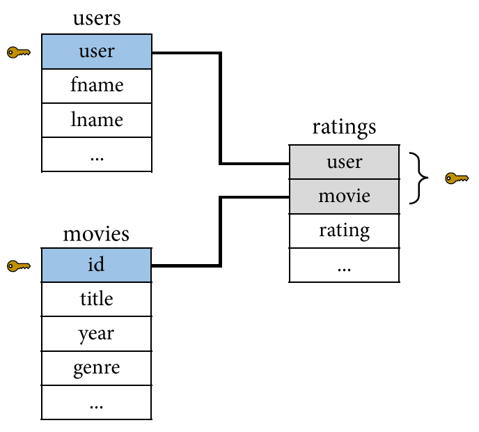
Data is relational when one observation references another observation
Each observation needs to be uniquely identified by one or more variables
- These variables are called “keys”
Natural keys are meaningful
- e.g., users$user
Surrogate keys are meaningless
- e.g., movies$id
The ratings table has a double-key

Complex Databases

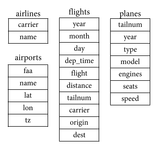
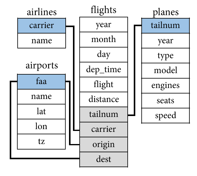
Let’s try to guess the connections for the {nycflights13} package’s tables

Basic Join Types

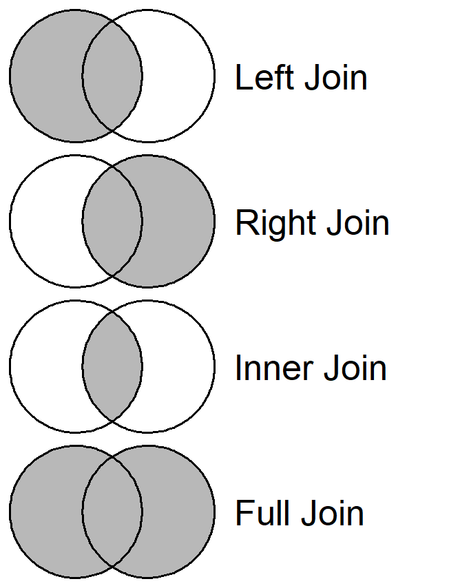
The basic joins handle non-overlapping or missing observations differently

movies

movie	year
1	2020
2	2003
3	2019
4	2006
5	2003
6	2002

avg_ratings

movie	average
2	2.2
3	8.0
4	6.7
5	8.7
6	3.5
7	7.5

Left Join

Left join includes all rows in the [left] table; those missing in the [right] table get NA

movies

movie	year
1	2020
2	2003
3	2019
4	2006
5	2003
6	2002

avg_ratings

movie	average
2	2.2
3	8.0
4	6.7
5	8.7
6	3.5
7	7.5

Left Join (movies, avg_ratings)

movie	year	average
1	2020	NA
2	2003	2.2
3	2019	8.0
4	2006	6.7
5	2003	8.7
6	2002	3.5

Right Join

Right join includes all rows in the [right] table; those missing in the [left] table get NA

movies

movie	year
1	2020
2	2003
3	2019
4	2006
5	2003
6	2002

avg_ratings

movie	average
2	2.2
3	8.0
4	6.7
5	8.7
6	3.5
7	7.5

Right Join (movies, avg_ratings)

movie	year	average
2	2003	2.2
3	2019	8.0
4	2006	6.7
5	2003	8.7
6	2002	3.5
7	NA	7.5

Inner Join

Inner join includes only rows present in both the [left] and [right] tables; no new NAs

movies

movie	year
1	2020
2	2003
3	2019
4	2006
5	2003
6	2002

avg_ratings

movie	average
2	2.2
3	8.0
4	6.7
5	8.7
6	3.5
7	7.5

Inner Join (movies, avg_ratings)

movie	year	average
2	2003	2.2
3	2019	8.0
4	2006	6.7
5	2003	8.7
6	2002	3.5

Full Join

Full join includes all rows in either the [left] or [right] table; missing values become NAs

movies

movie	year
1	2020
2	2003
3	2019
4	2006
5	2003
6	2002

avg_ratings

movie	average
2	2.2
3	8.0
4	6.7
5	8.7
6	3.5
7	7.5

Full Join (movies, avg_ratings)

movie	year	average
1	2020	NA
2	2003	2.2
3	2019	8.0
4	2006	6.7
5	2003	8.7
6	2002	3.5
7	NA	7.5

Tidyverse Joins

{dplyr} has intuitive, standard names for these concepts
- left_join(x, y, by)
- right_join(x, y, by)
- inner_join(x, y, by)
- full_join(x, y, by)
It is easiest if the key variables have the same names in both tibbles
- e.g., by = "carrier"
- e.g., by = c("user", "movie")
But you can join by differently named keys too
- e.g., by = join_by(faa == origin)

Preparing our Data

Let’s examine a subset of columns from flights.

data("flights", package = "nycflights13")

flights2 <- 
  flights |> 
  select(month, day, flight, origin, dest, tailnum, carrier) |> 
  print()

# A tibble: 336,776 × 7
  month   day flight origin dest  tailnum carrier
  <int> <int>  <int> <chr>  <chr> <chr>   <chr>  
1     1     1   1545 EWR    IAH   N14228  UA     
2     1     1   1714 LGA    IAH   N24211  UA     
3     1     1   1141 JFK    MIA   N619AA  AA     
4     1     1    725 JFK    BQN   N804JB  B6     
5     1     1    461 LGA    ATL   N668DN  DL     
# ℹ 336,771 more rows

The Airlines Dataset

Before we join, let’s look at the airlines dataset.

data("airlines", package = "nycflights13")

airlines

# A tibble: 16 × 2
  carrier name                  
  <chr>   <chr>                 
1 9E      Endeavor Air Inc.     
2 AA      American Airlines Inc.
3 AS      Alaska Airlines Inc.  
4 B6      JetBlue Airways       
5 DL      Delta Air Lines Inc.  
# ℹ 11 more rows

Left Join in R

Question: What is the full name of the airline carrier for each flight?

A left join is perfect for looking up and adding reference information to our primary dataset. Notice that the number of rows remains exactly the same.

flights2 |> 
  left_join(airlines, by = "carrier")

# A tibble: 336,776 × 8
  month   day flight origin dest  tailnum carrier name                  
  <int> <int>  <int> <chr>  <chr> <chr>   <chr>   <chr>                 
1     1     1   1545 EWR    IAH   N14228  UA      United Air Lines Inc. 
2     1     1   1714 LGA    IAH   N24211  UA      United Air Lines Inc. 
3     1     1   1141 JFK    MIA   N619AA  AA      American Airlines Inc.
4     1     1    725 JFK    BQN   N804JB  B6      JetBlue Airways       
5     1     1    461 LGA    ATL   N668DN  DL      Delta Air Lines Inc.  
# ℹ 336,771 more rows

The Airports Dataset

Next, let’s select a few columns from airports.

data("airports", package = "nycflights13")

airports2 <- 
  airports |> 
  select(faa, name) |> 
  print()

# A tibble: 1,458 × 2
  faa   name                         
  <chr> <chr>                        
1 04G   Lansdowne Airport            
2 06A   Moton Field Municipal Airport
3 06C   Schaumburg Regional          
4 06N   Randall Airport              
5 09J   Jekyll Island Airport        
# ℹ 1,453 more rows

Joining by Different Names

If the key variables are named differently across datasets, we provide by with the join_by() function. The order should match first == second.

flights2 |> 
  left_join(airports2, by = join_by(origin == faa))

# A tibble: 336,776 × 8
  month   day flight origin dest  tailnum carrier name               
  <int> <int>  <int> <chr>  <chr> <chr>   <chr>   <chr>              
1     1     1   1545 EWR    IAH   N14228  UA      Newark Liberty Intl
2     1     1   1714 LGA    IAH   N24211  UA      La Guardia         
3     1     1   1141 JFK    MIA   N619AA  AA      John F Kennedy Intl
4     1     1    725 JFK    BQN   N804JB  B6      John F Kennedy Intl
5     1     1    461 LGA    ATL   N668DN  DL      La Guardia         
# ℹ 336,771 more rows

Duplicate Column Names

We now have the name.x (origin) and name.y (dest)…

flights2 |> 
  left_join(airports2, by = join_by(origin == faa)) |> 
  left_join(airports2, by = join_by(dest == faa))

# A tibble: 336,776 × 9
  month   day flight origin dest  tailnum carrier name.x              name.y    
  <int> <int>  <int> <chr>  <chr> <chr>   <chr>   <chr>               <chr>     
1     1     1   1545 EWR    IAH   N14228  UA      Newark Liberty Intl George Bu…
2     1     1   1714 LGA    IAH   N24211  UA      La Guardia          George Bu…
3     1     1   1141 JFK    MIA   N619AA  AA      John F Kennedy Intl Miami Intl
4     1     1    725 JFK    BQN   N804JB  B6      John F Kennedy Intl <NA>      
5     1     1    461 LGA    ATL   N668DN  DL      La Guardia          Hartsfiel…
# ℹ 336,771 more rows

Changing the Suffixes

We can replace “.x” and “.y” using suffix in the second join.

flights2 |> 
  left_join(airports2, by = join_by(origin == faa)) |> 
  left_join(airports2, by = join_by(dest == faa),
            suffix = c("_origin", "_dest"))

# A tibble: 336,776 × 9
  month   day flight origin dest  tailnum carrier name_origin         name_dest 
  <int> <int>  <int> <chr>  <chr> <chr>   <chr>   <chr>               <chr>     
1     1     1   1545 EWR    IAH   N14228  UA      Newark Liberty Intl George Bu…
2     1     1   1714 LGA    IAH   N24211  UA      La Guardia          George Bu…
3     1     1   1141 JFK    MIA   N619AA  AA      John F Kennedy Intl Miami Intl
4     1     1    725 JFK    BQN   N804JB  B6      John F Kennedy Intl <NA>      
5     1     1    461 LGA    ATL   N668DN  DL      La Guardia          Hartsfiel…
# ℹ 336,771 more rows

The Planes Dataset

Finally, let’s select a few columns from planes.

data("planes", package = "nycflights13")

planes2 <- 
  planes |> 
  select(tailnum, manufacturer, model) |> 
  print()

# A tibble: 3,322 × 3
  tailnum manufacturer     model    
  <chr>   <chr>            <chr>    
1 N10156  EMBRAER          EMB-145XR
2 N102UW  AIRBUS INDUSTRIE A320-214 
3 N103US  AIRBUS INDUSTRIE A320-214 
4 N104UW  AIRBUS INDUSTRIE A320-214 
5 N10575  EMBRAER          EMB-145LR
# ℹ 3,317 more rows

Missing Matches

If flights2 has a key that does not exist in the right dataset, the joined variables become NA. Let’s look at plane “N3ALAA” to see this in action.

flights2 |> 
  left_join(planes2, by = "tailnum") |> 
  filter(tailnum == "N3ALAA")

# A tibble: 63 × 9
  month   day flight origin dest  tailnum carrier manufacturer model
  <int> <int>  <int> <chr>  <chr> <chr>   <chr>   <chr>        <chr>
1     1     1    301 LGA    ORD   N3ALAA  AA      <NA>         <NA> 
2     1     2    353 LGA    ORD   N3ALAA  AA      <NA>         <NA> 
3     1     3    301 LGA    ORD   N3ALAA  AA      <NA>         <NA> 
4     1     7    359 LGA    ORD   N3ALAA  AA      <NA>         <NA> 
5     1     8   1351 JFK    ORD   N3ALAA  AA      <NA>         <NA> 
# ℹ 58 more rows

Inner Join in R

Question: Which flights were flown by planes that we have registry data for?

To only return rows that have a match in both tables, use inner join. Our row count will decrease because it drops flights with missing plane data.

flights2 |> 
  inner_join(planes2, by = "tailnum")

# A tibble: 284,170 × 9
  month   day flight origin dest  tailnum carrier manufacturer model   
  <int> <int>  <int> <chr>  <chr> <chr>   <chr>   <chr>        <chr>   
1     1     1   1545 EWR    IAH   N14228  UA      BOEING       737-824 
2     1     1   1714 LGA    IAH   N24211  UA      BOEING       737-824 
3     1     1   1141 JFK    MIA   N619AA  AA      BOEING       757-223 
4     1     1    725 JFK    BQN   N804JB  B6      AIRBUS       A320-232
5     1     1    461 LGA    ATL   N668DN  DL      BOEING       757-232 
# ℹ 284,165 more rows

Right Join in R

Question: Which airports in our data received zero flights from NYC in 2013?

A right join is useful when we want to keep all observations from a reference table on the right without breaking the flow of our code.

flights2 |> 
  right_join(airports2, by = join_by(dest == faa)) |> 
  filter(is.na(flight)) |> 
  select(dest, name)

# A tibble: 1,357 × 2
  dest  name                         
  <chr> <chr>                        
1 04G   Lansdowne Airport            
2 06A   Moton Field Municipal Airport
3 06C   Schaumburg Regional          
4 06N   Randall Airport              
5 09J   Jekyll Island Airport        
# ℹ 1,352 more rows

Full Join in R

Question: Overall, how many flights went to unlisted airports, and how many listed airports received zero flights?

A full join keeps all rows from both tables. By joining flights with airports, we can audit the overlaps and missing matches across our entire database.

flights2 |> 
  full_join(airports2, by = join_by(dest == faa)) |> 
  count(
    missing_airport = is.na(name),
    missing_flight = is.na(flight)
  )

# A tibble: 3 × 3
  missing_airport missing_flight      n
  <lgl>           <lgl>           <int>
1 FALSE           FALSE          329174
2 FALSE           TRUE             1357
3 TRUE            FALSE            7602

Foundations of Data Science

Roadmap

Relational Data

Relational Data

Relational Data

Keys

Complex Databases

Basic Join Types

Basic Join Types

Left Join

Right Join

Inner Join

Full Join

Tidyverse Joins

Tidyverse Joins

Preparing our Data

The Airlines Dataset

Left Join in R

The Airports Dataset

Joining by Different Names

Duplicate Column Names

Changing the Suffixes

The Planes Dataset

Missing Matches

Inner Join in R

Right Join in R

Full Join in R

Foundations of
Data Science