Foundations of
Data Science

Spring 2026 | Data 2 (399)
Jeffrey M. Girard | Lecture 12b

Roadmap

• Understand the difference between character strings and factors

• Control the order of categorical data in plots and tables

• Recode, collapse, and “lump” factor levels to simplify messy data

Creating Factors

What are Factors?

• Question: Why not just use strings for categories?

• Factors are used for categorical variables with a fixed and known set of possible values (levels)

• Each level can also have a nice display label

• Unlike strings, factors allow you to control the order of categories and check for invalid values

• We use the {forcats} package (part of the {tidyverse}) to work with them
• Most functions in this package start with fct_

Creating Factors

Question: How do we convert raw data into a factor?

# Raw data as numbers (where 1=Female, 2=Male and 11 is a typo)
sex <- c(2, 1, 1, 2, 11)

# Convert to factor so R knows that only 1 and 2 were valid
fct_sex <- factor(sex, levels = c(1, 2))
fct_sex

[1] 2    1    1    2    <NA>
Levels: 1 2

# Each level can be given a string to serve as its "label"
factor(sex, levels = c(1, 2), labels = c("Female", "Male"))

[1] Male   Female Female Male   <NA>  
Levels: Female Male

Factors vs. Strings

Question: What happens if we don’t specify levels?

# Raw data as strings
birth_months <- c("Jan", "Feb", "Feb", "Jan", "Apr", "Mar", "Apr")

# Default levels = observed values in alphanumeric order
factor(birth_months)

[1] Jan Feb Feb Jan Apr Mar Apr
Levels: Apr Feb Jan Mar

# Explicitly define levels and order (including unobserved ones)
factor(birth_months, levels = c("Jan", "Feb", "Mar", "Apr", "May", "Jun", 
                                "Jul", "Aug", "Sep", "Oct", "Nov", "Dec"))

[1] Jan Feb Feb Jan Apr Mar Apr
Levels: Jan Feb Mar Apr May Jun Jul Aug Sep Oct Nov Dec

A Safer Alternative

Question: Are there better tools for creating factors than base R?

The {forcats} package provides fct(). It is safer than factor() because it errors if you include a value not in the levels, and it orders by first appearance.

# Base R factor() silently creates NAs for typos
factor(c("Dec", "Apr", "Jam", "Mar"), levels = c("Jan", "Feb", "Mar", "Apr", "Dec"))

[1] Dec  Apr  <NA> Mar 
Levels: Jan Feb Mar Apr Dec

# forcats::fct() catches the error for us
fct(c("Dec", "Apr", "Jam", "Mar"), levels = c("Jan", "Feb", "Mar", "Apr", "Dec"))

Error in `fct()`:
! All values of `x` must appear in `levels` or `na`
ℹ Missing level: "Jam"

Ordering Levels

Introducing the GSS Dataset

To explore reordering and modifying factors, we will use the gss_cat dataset. This is a sample of data from the General Social Survey.

library(tidyverse)
data("gss_cat", package = "forcats")
glimpse(gss_cat)

Rows: 21,483
Columns: 9
$ year    <int> 2000, 2000, 2000, 2000, 2000, 2000, 2000, 2000, 2000, 2000, 20…
$ marital <fct> Never married, Divorced, Widowed, Never married, Divorced, Mar…
$ age     <int> 26, 48, 67, 39, 25, 25, 36, 44, 44, 47, 53, 52, 52, 51, 52, 40…
$ race    <fct> White, White, White, White, White, White, White, White, White,…
$ rincome <fct> $8000 to 9999, $8000 to 9999, Not applicable, Not applicable, …
$ partyid <fct> "Ind,near rep", "Not str republican", "Independent", "Ind,near…
$ relig   <fct> Protestant, Protestant, Protestant, Orthodox-christian, None, …
$ denom   <fct> "Southern baptist", "Baptist-dk which", "No denomination", "No…
$ tvhours <int> 12, NA, 2, 4, 1, NA, 3, NA, 0, 3, 2, NA, 1, NA, 1, 7, NA, 3, 3…

Order by Appearance

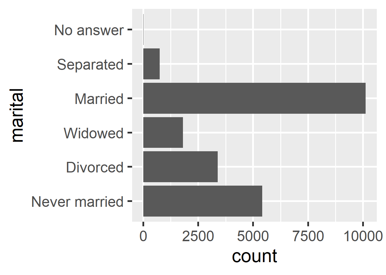
Question: Can I order my levels by which appear first in the data?

gss_cat |> 
  mutate(
    marital = fct_inorder(marital)
  ) |> 
  ggplot(aes(y = marital)) + 
  geom_bar()

Order by Frequency

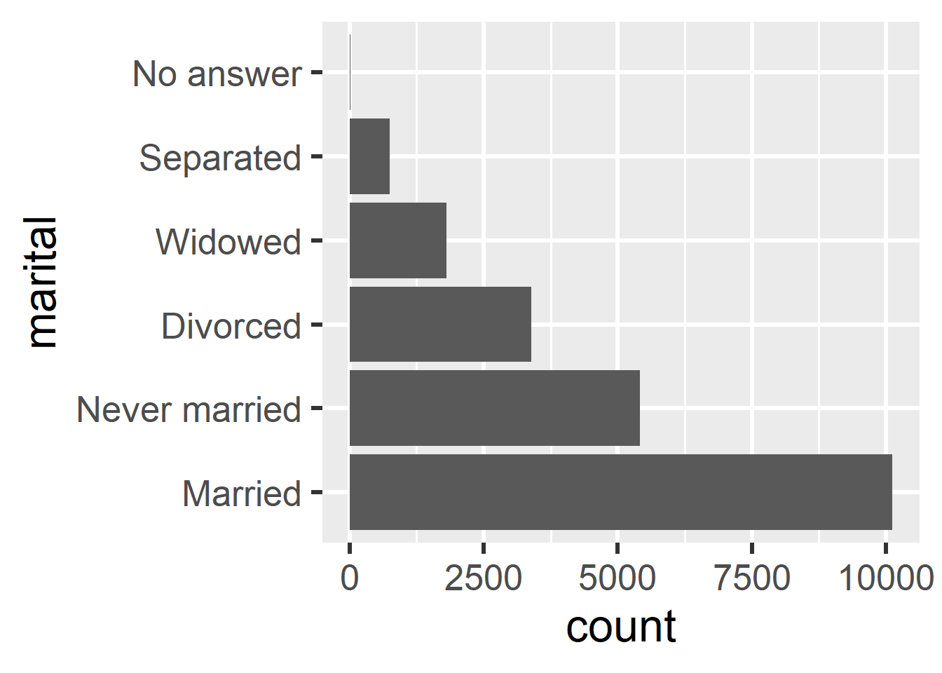
Question: How can I order my levels by their number of observations?

gss_cat |> 
  mutate(
    marital = fct_infreq(marital)
  ) |> 
  ggplot(aes(y = marital)) + 
  geom_bar()

Reversing Order

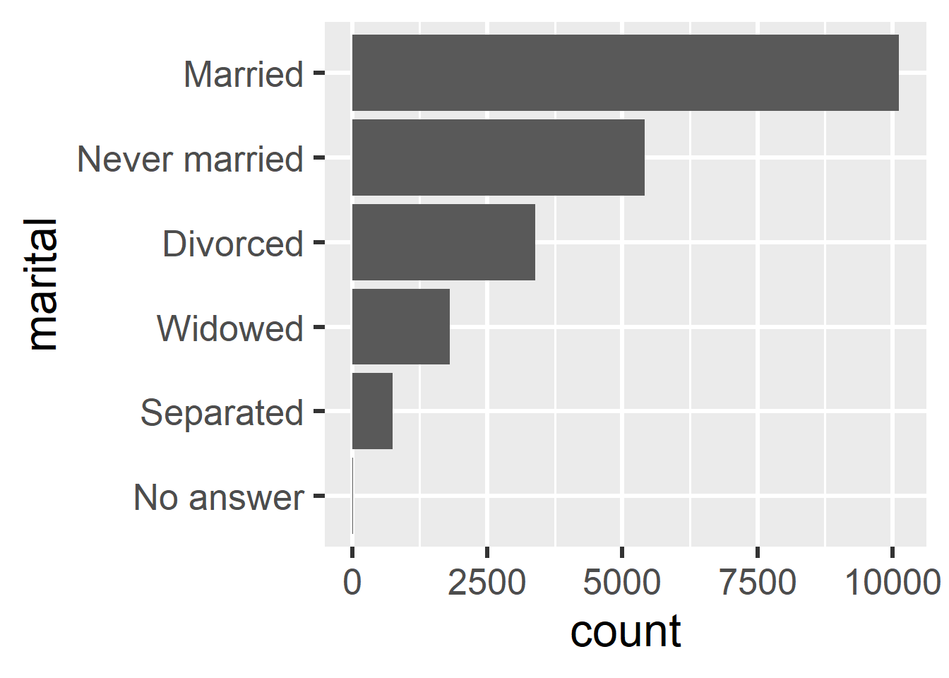
Question: Can I quickly reverse the order of my factors?

gss_cat |> 
  mutate( 
    marital = 
      marital |> 
      fct_infreq() |> 
      fct_rev()
  ) |> 
  ggplot(aes(y = marital)) + 
  geom_bar()

Creating a Summary Table

Let’s calculate the average age for each marital status group to play with.

gss_age <- gss_cat |> 
  drop_na(age) |> 
  summarize(
    .by = marital,
    mean_age = mean(age)
  ) |> 
  print()

# A tibble: 6 × 2
  marital       mean_age
  <fct>            <dbl>
1 Never married     33.9
2 Divorced          51.1
3 Widowed           71.7
4 Married           48.7
5 Separated         45.3
6 No answer         52.4

Order by Value

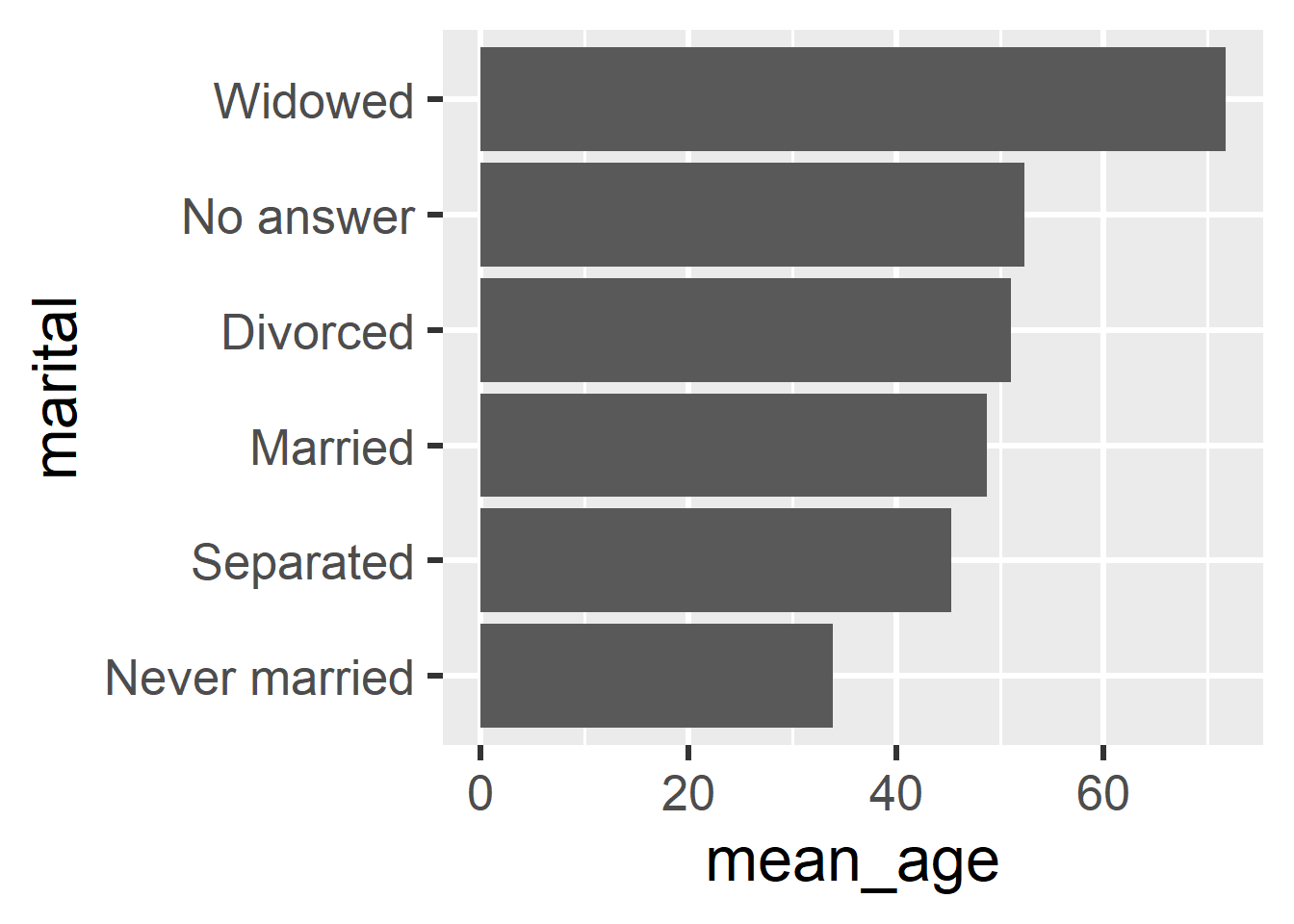
Order by another variable in the dataset

# Order by average age
gss_age |> 
  mutate(
    marital = fct_reorder(
      marital,  # factor to reorder
      mean_age  # values to order by
    )
  ) |> 
  ggplot(
    aes(
      x = mean_age, 
      y = marital
    )
  ) + 
  geom_col()

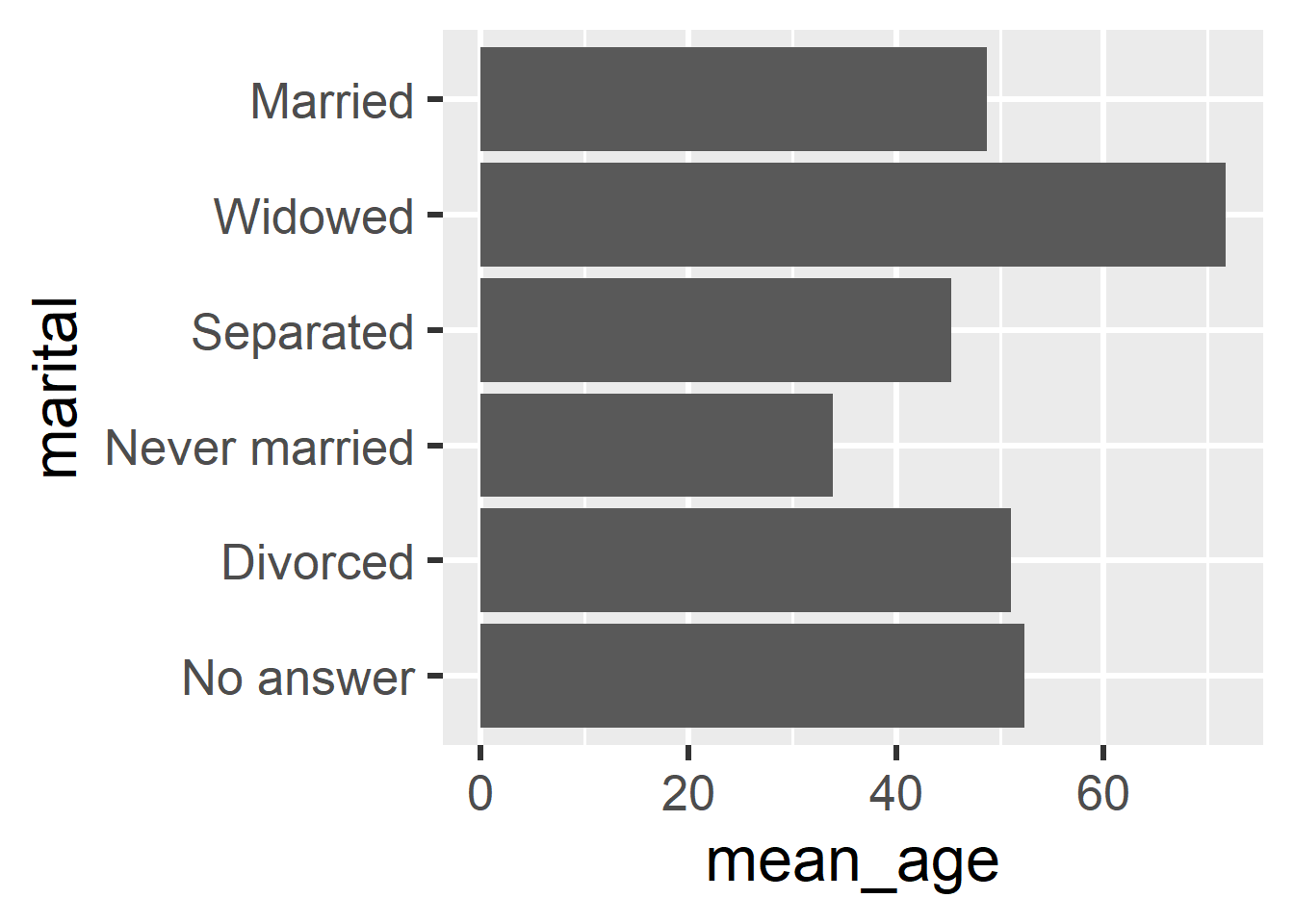
Manual Reordering

Manually bring one or more variables to the front / bottom

gss_age |> 
  mutate(
    marital = fct_relevel(
      marital,
      "No answer", # first
      "Divorced"   # second
    )
  ) |> 
  ggplot(aes(
    x = mean_age,
    y = marital
  )) + 
  geom_col()

Modifying Levels

Why Modify Levels?

• Sometimes the data you inherit has messy categories
• You might need to combine small, specific groups into larger, more general ones for analysis
• Categorical variables with too many levels can cause issues
• Modifying levels allows us to tidy up before plotting or modeling

Recoding Levels

Question: How do we rename levels to make them clearer?

gss_cat |> 
  mutate(partyid = fct_recode(partyid,
    "rep, strong" = "Strong republican",
    "rep, weak"  = "Not str republican",
    "ind, rep" = "Ind,near rep",
    "ind"  = "Independent",
    "ind, dem" = "Ind,near dem",
    "dem, weak"  = "Not str democrat",
    "dem, strong" = "Strong democrat"
  )) |> 
  count(partyid) |> 
  print(n = 10)

# A tibble: 10 × 2
   partyid         n
   <fct>       <int>
 1 No answer     154
 2 Don't know      1
 3 Other party   393
 4 rep, strong  2314
 5 rep, weak    3032
 6 ind, rep     1791
 7 ind          4119
 8 ind, dem     2499
 9 dem, weak    3690
10 dem, strong  3490

Collapsing Levels

Question: How do we group many small categories into a few large ones?

gss_cat |> 
  mutate(party_simple = fct_collapse(partyid,
    other = c("No answer", "Don't know", "Other party"),
    rep   = c("Strong republican", "Not str republican"),
    ind   = c("Ind,near rep", "Independent", "Ind,near dem"),
    dem   = c("Not str democrat", "Strong democrat")
  )) |> 
  count(party_simple, sort = TRUE)

# A tibble: 4 × 2
  party_simple     n
  <fct>        <int>
1 ind           8409
2 dem           7180
3 rep           5346
4 other          548

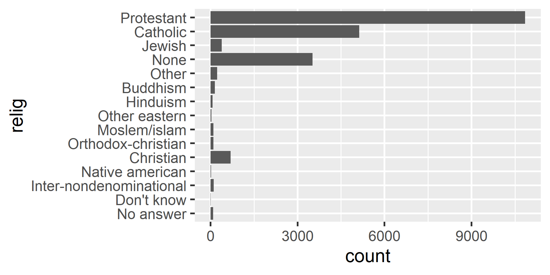
Many Small Groups

gss_cat |> ggplot(aes(y = relig)) + geom_bar()

Lumping Small Groups

Question: What if we only care about the most common categories?

gss_cat |> 
  mutate(
    # Keep the 5 largest religions and lump all others
    relig_lumped = fct_lump_n(relig, n = 5)
  ) |> 
  count(relig_lumped, sort = TRUE)

# A tibble: 6 × 2
  relig_lumped     n
  <fct>        <int>
1 Protestant   10846
2 Catholic      5124
3 None          3523
4 Other          913
5 Christian      689
6 Jewish         388

Other Ways to Lump

Question: What if I want to lump based on proportions rather than a fixed count?

gss_cat |> 
  mutate(
    # Keep religions that appear at least 5% of the time
    relig_prop = fct_lump_prop(relig, prop = 0.05)
  ) |> 
  count(relig_prop, sort = TRUE)

# A tibble: 4 × 2
  relig_prop     n
  <fct>      <int>
1 Protestant 10846
2 Catholic    5124
3 None        3523
4 Other       1990