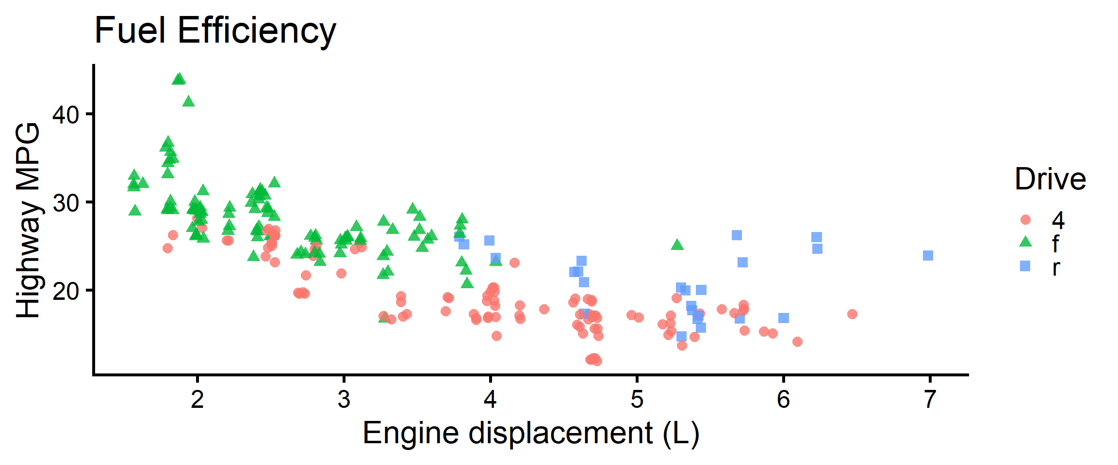
# theme_classic() removes gridlines and gives a clean axis
p + theme_classic(base_size = 24)Foundations of
Data Science
Spring 2026 | Data 2 (399)
Jeffrey M. Girard | Lecture 13c

Setup for Themes
library(tidyverse)
# Create a base plot to add themes to
p <-
  ggplot(mpg, aes(x = displ, y = hwy)) +
  geom_jitter(
    aes(color = drv, shape = drv),
    size = 3, alpha = 0.8
  ) +
  labs(
    x = "Engine displacement (L)",
    y = "Highway MPG",
    color = "Drive",
    shape = "Drive",
    title = "Fuel Efficiency"
  )

p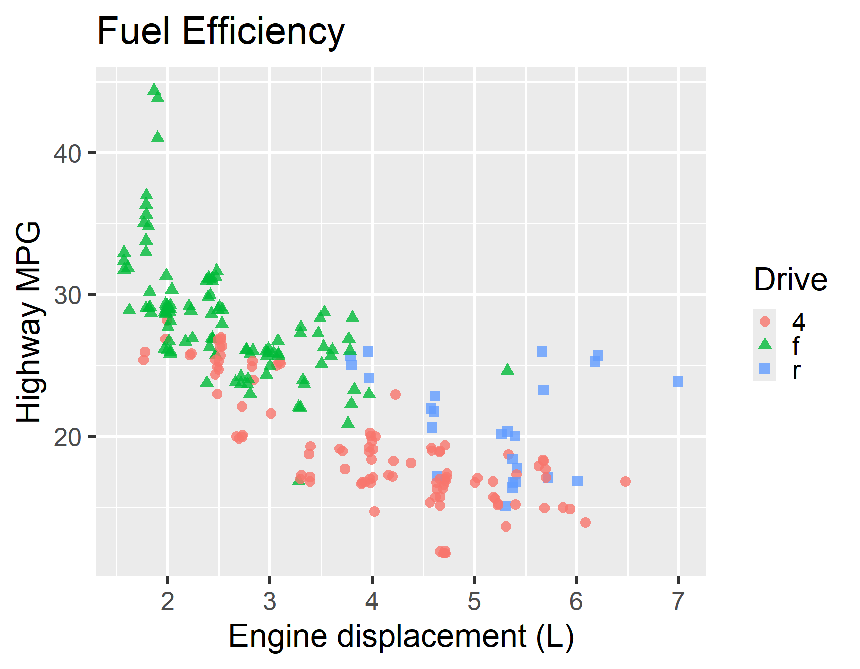
Classic Theme
Black and White Theme
# theme_bw() adds a border and keeps major gridlines
p + theme_bw(base_size = 24)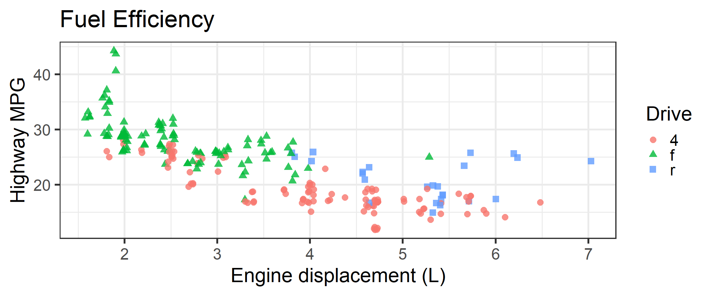
Minimal Theme
# theme_minimal() removes the background box for a modern look
p + theme_minimal(base_size = 24)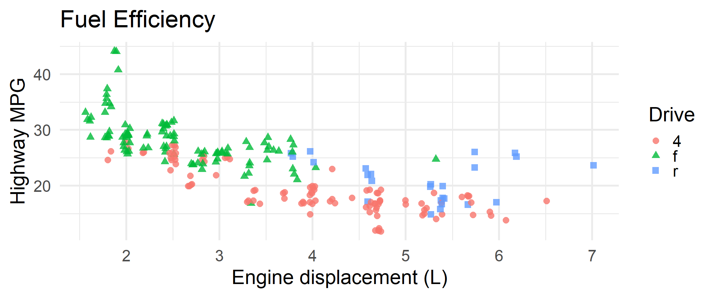
Legend Position
# Move the legend to the bottom, top, left, or "none"
p + theme(legend.position = "bottom")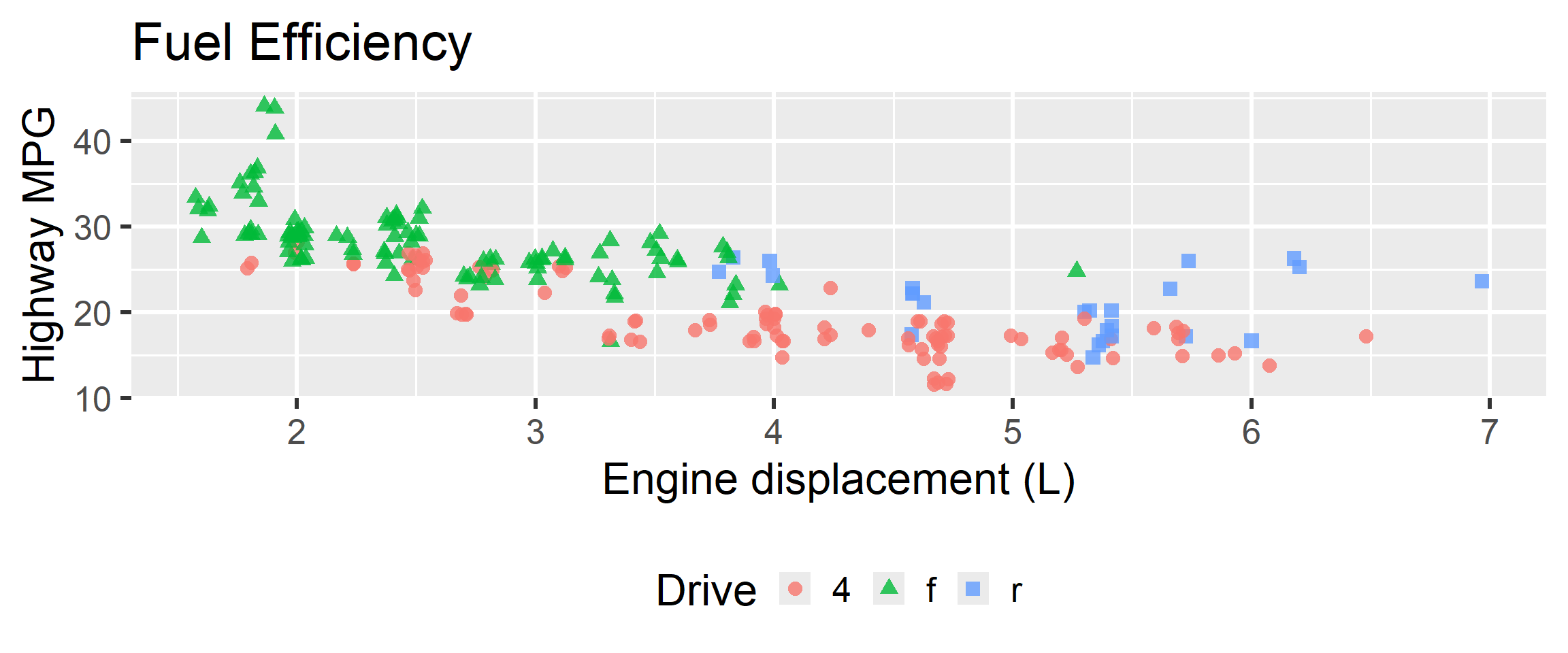
Legend Coordinates
# Move the legend inside the plot using relative coordinates (0 to 1)
p + theme(legend.position = c(0.85, 0.8))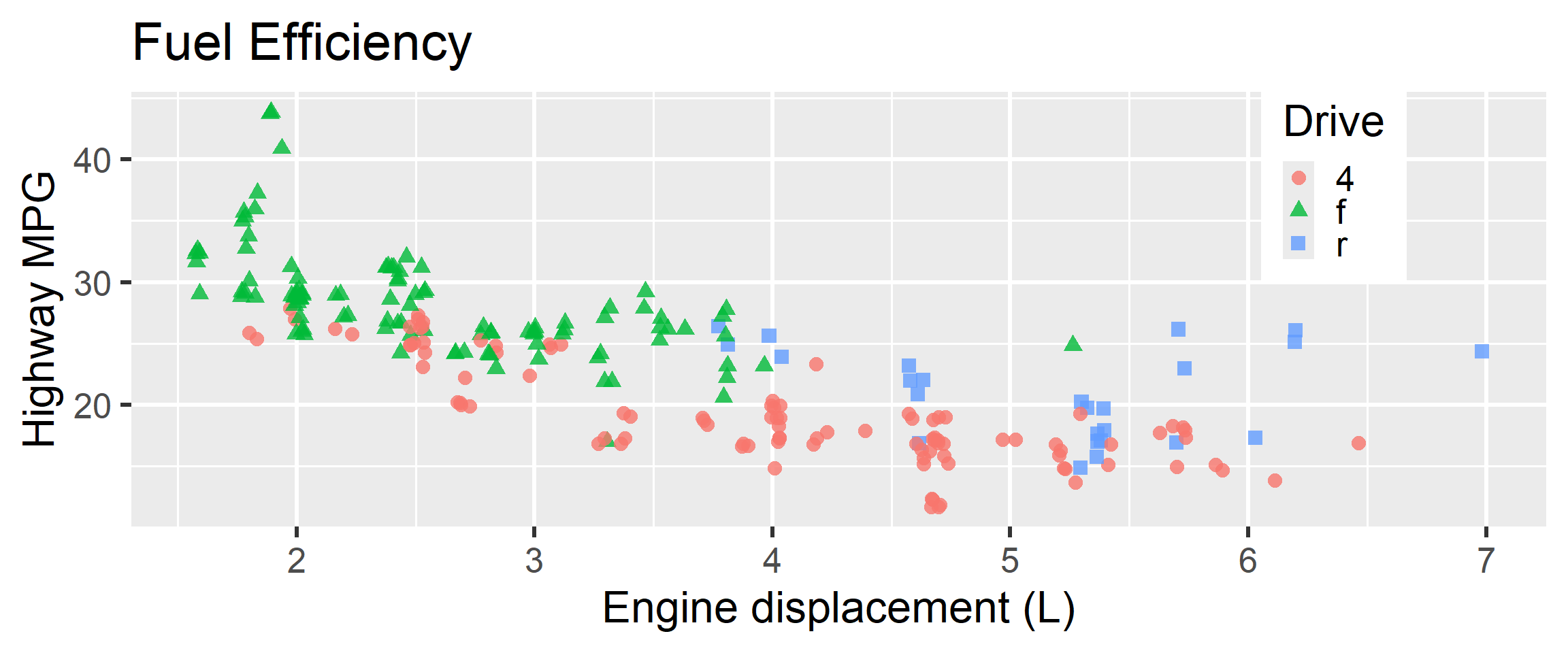
Text Elements
# Use element_text() to change font properties
p + theme(plot.title = element_text(face = "bold", color = "red"))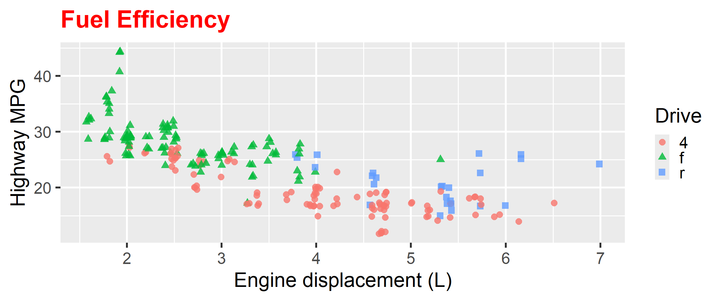
Line Elements
# Use element_line() to modify gridlines and axes
p + theme(panel.grid.major = element_line(linetype = "dashed", color = "red"))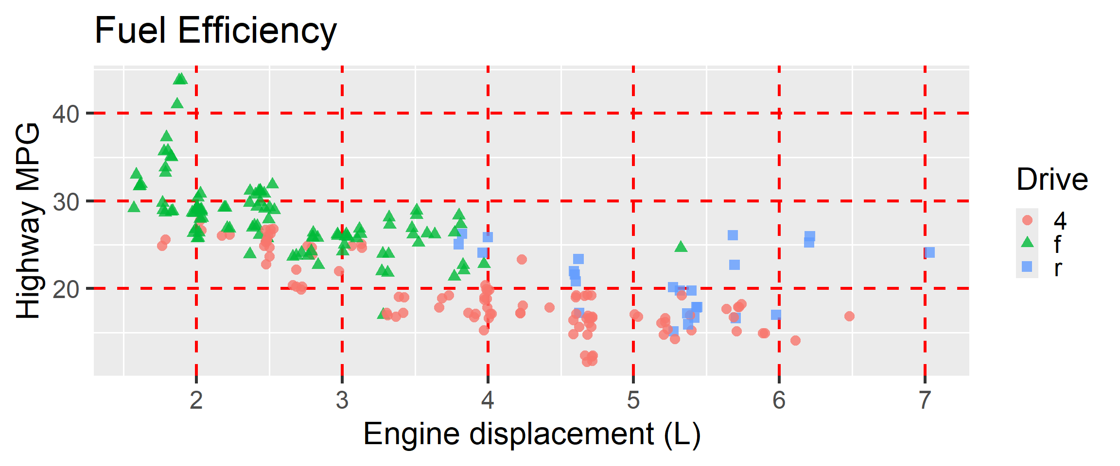
Blanking
# Use element_blank() to remove specific features entirely
p + theme(panel.grid.minor = element_blank(), axis.ticks.x = element_blank())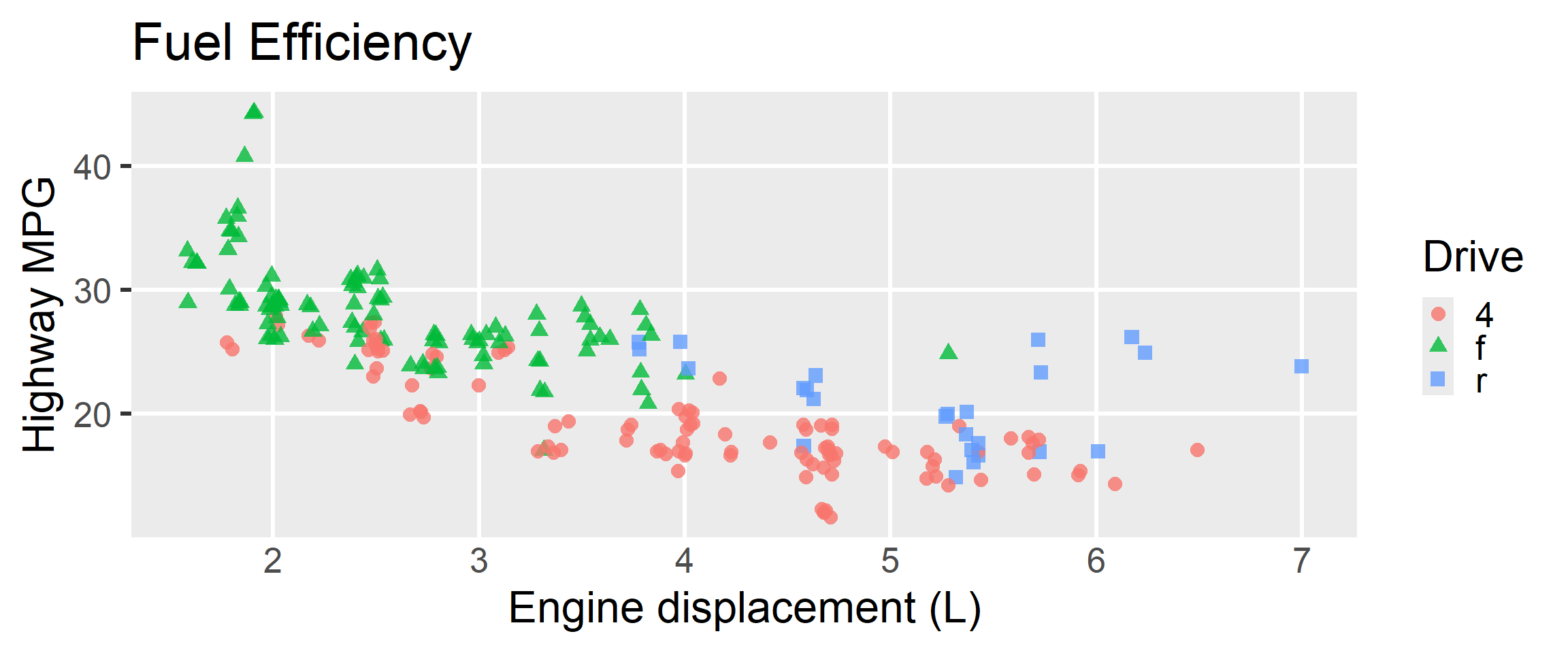
Reusable Themes
# Store your custom theme in an object
# Then apply it to multiple plots
my_theme <-
  theme_minimal(base_size = 30) +
  theme(
    legend.position = "bottom",
    plot.title =
      element_text(face = "bold"),
    panel.grid.minor = element_blank()
  )

p + my_theme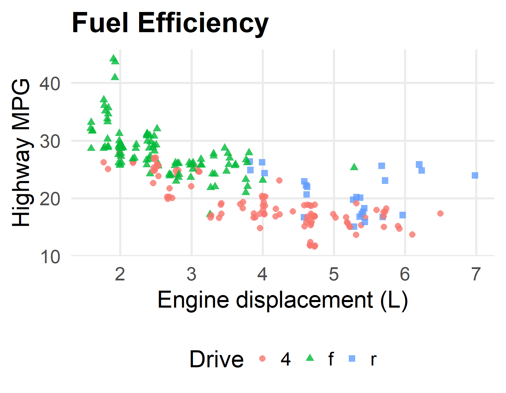
Combining Plots: Basic Addition
# The + operator attempts to lay out the plots logically
library(patchwork)

p1 + p2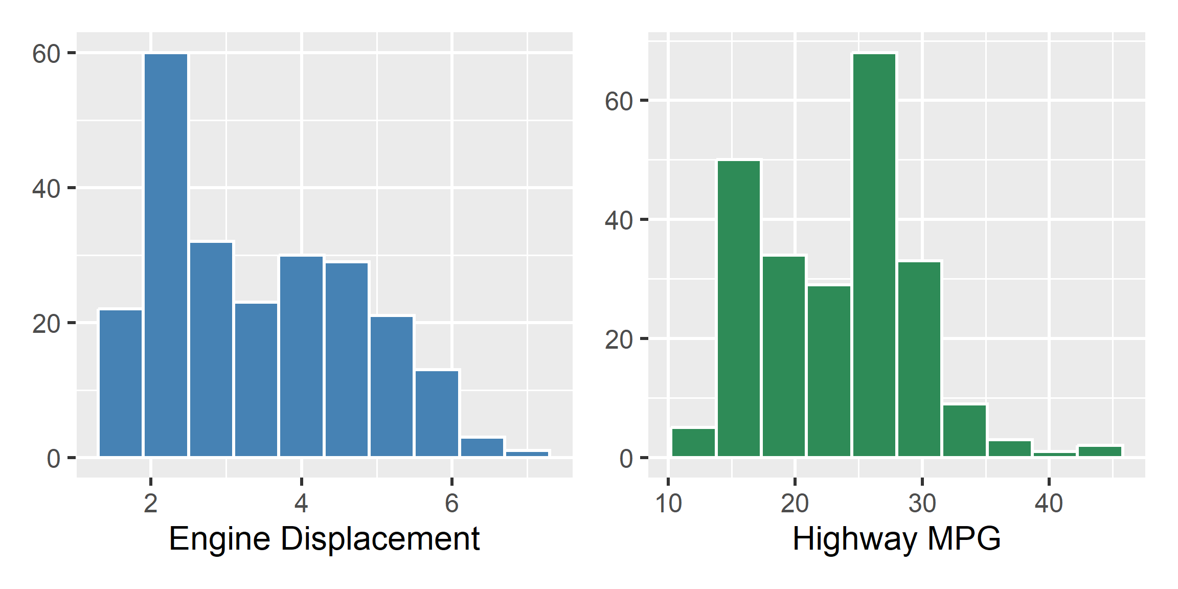
Controlling the Layout
# Use plot_layout() to explicitly state columns or rows
p1 + p2 + p3 + plot_layout(ncol = 3)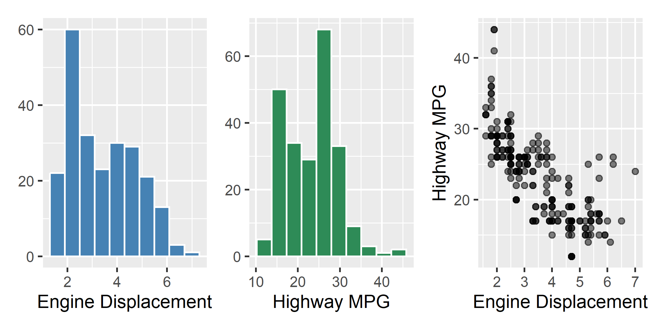
Adding Spacers
# Use plot_spacer() to leave empty areas in the grid
p1 + plot_spacer() + p2 + plot_layout(ncol = 3)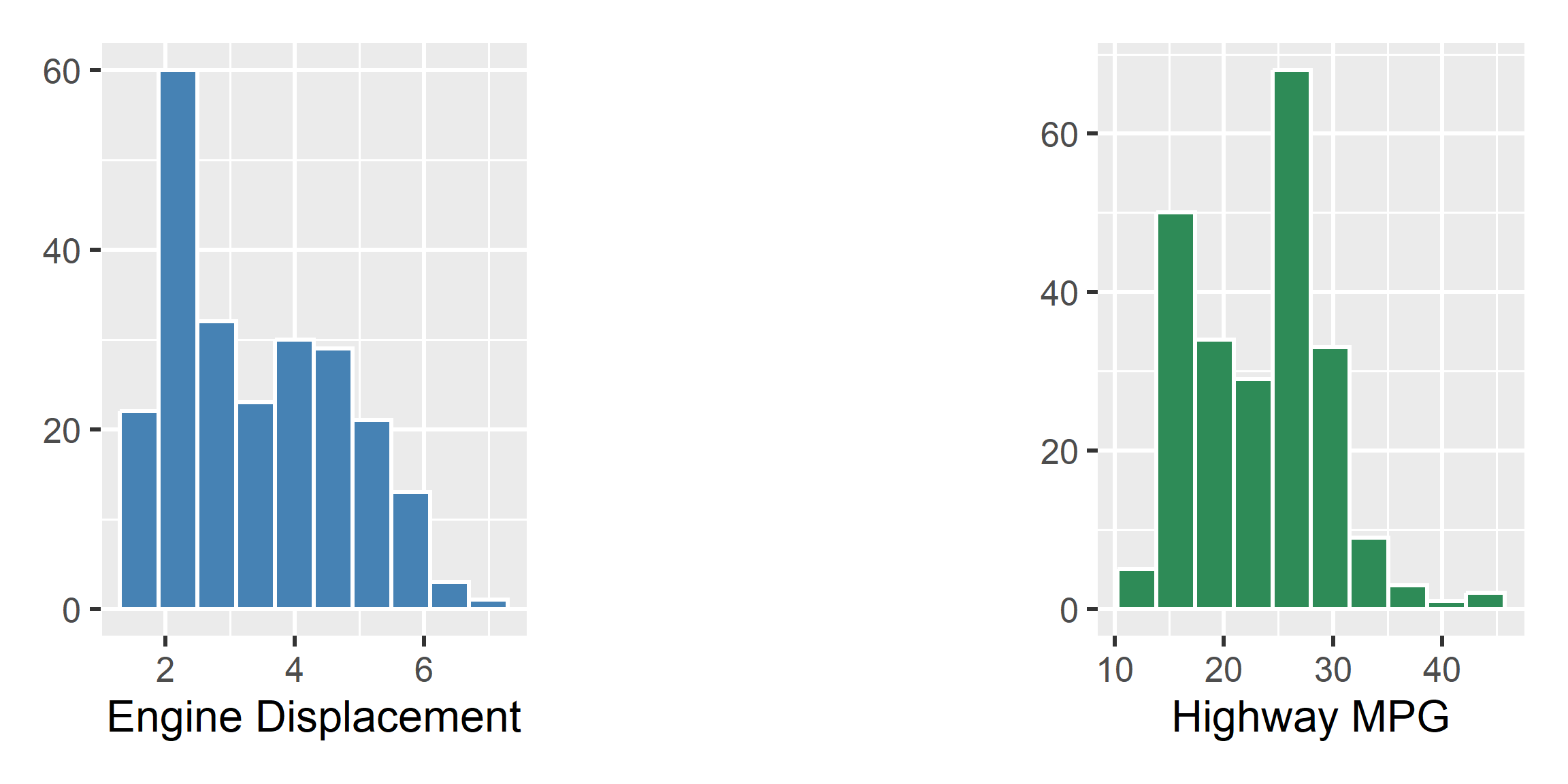
Side-by-Side
# The | operator explicitly places plots side-by-side
p1 | p2 | p3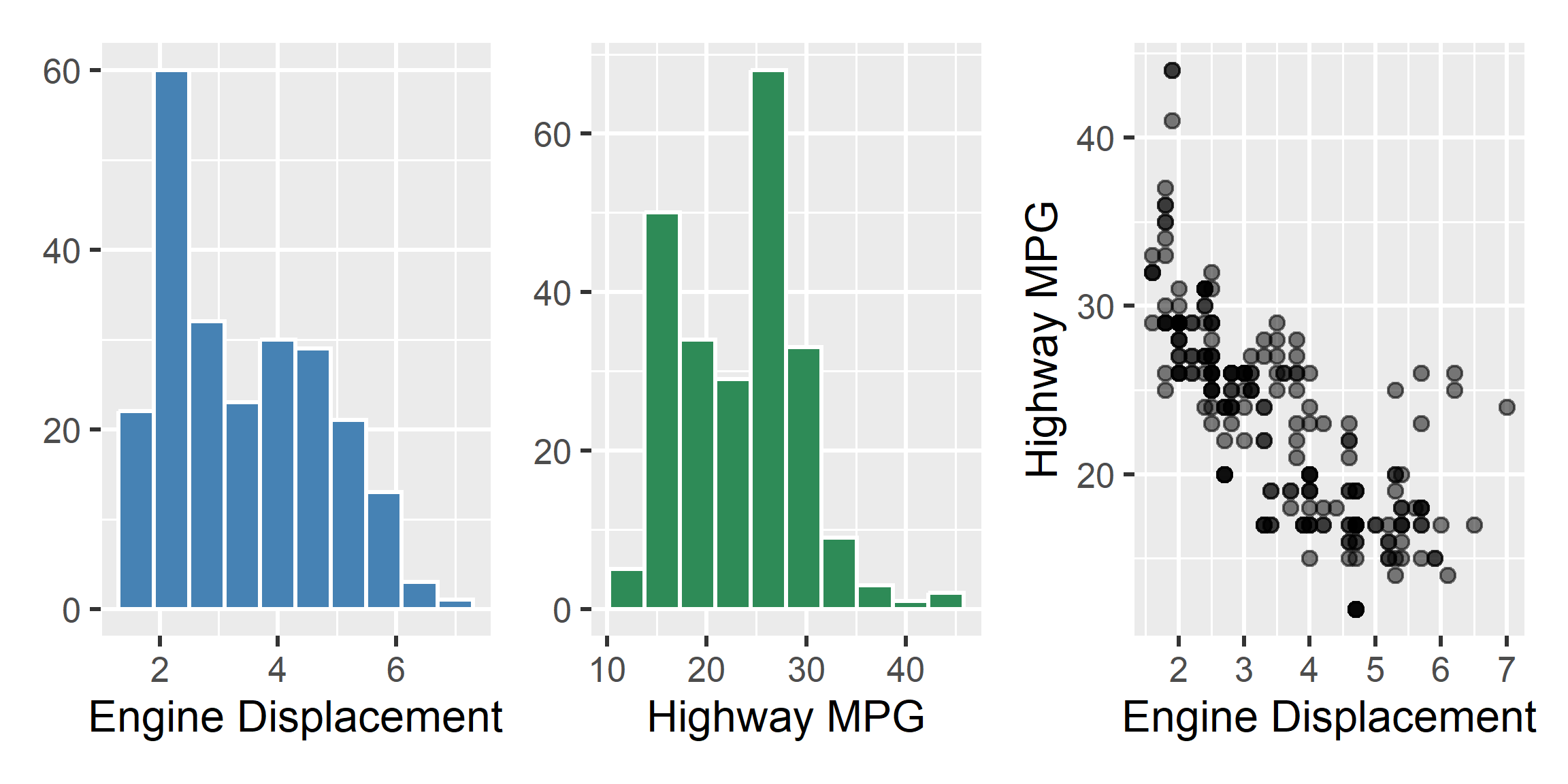
Above-and-Below
# The / operator explicitly places plots above and below
p1 / p3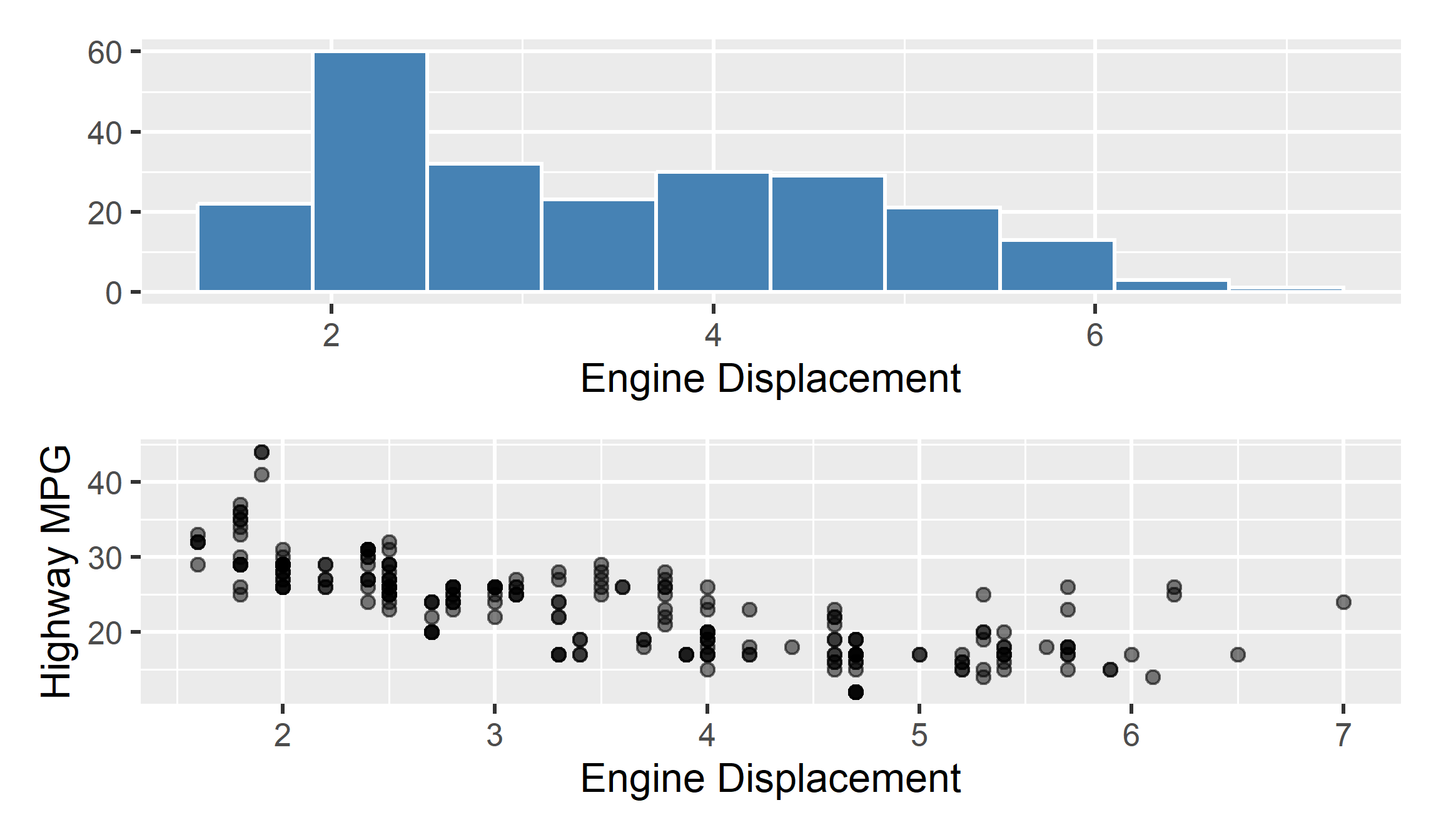
Mixing and Matching
# Parentheses determine nesting and grouping
(p1 | p2) / p3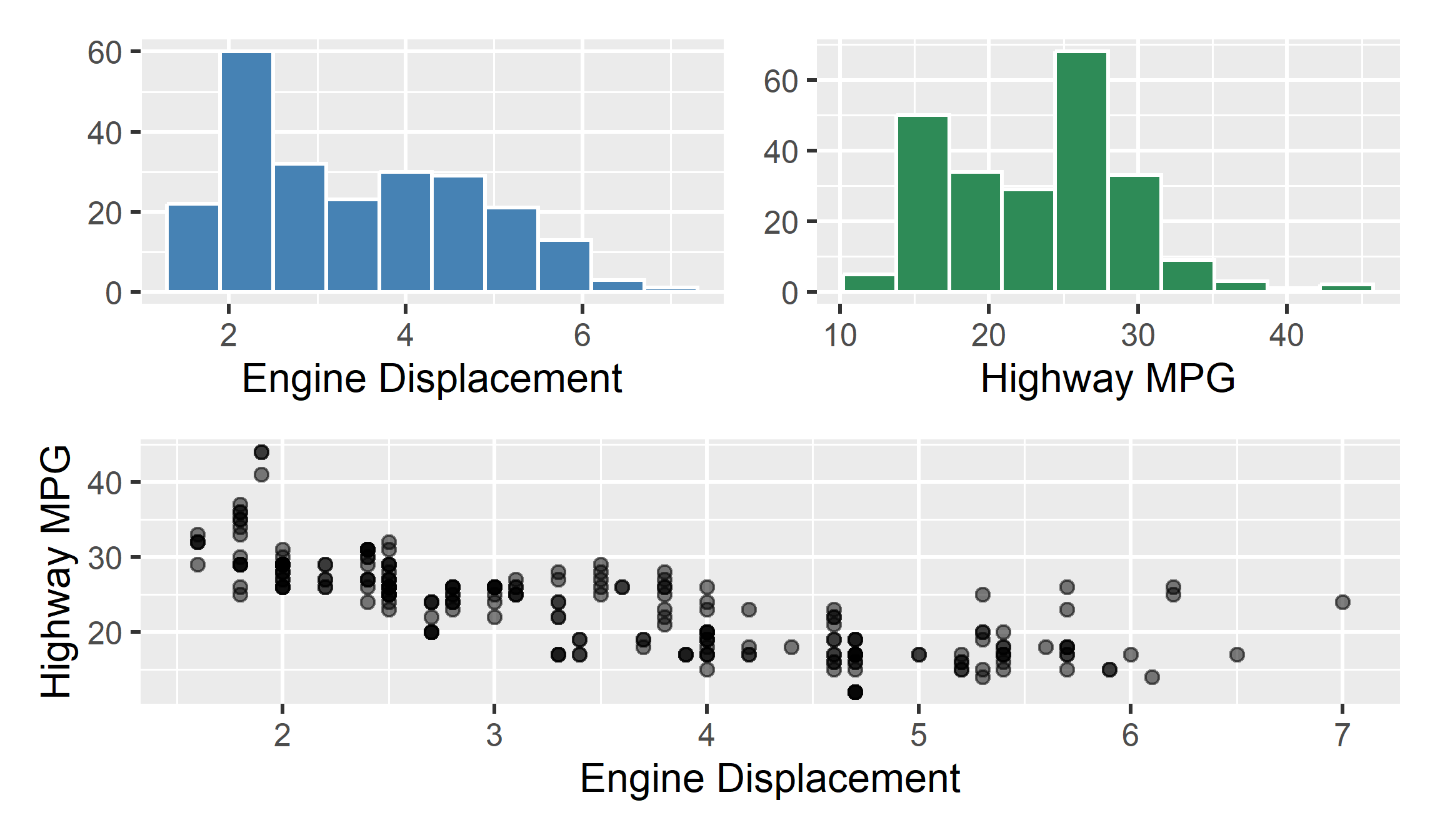
Relative Sizes
# Pass a vector to widths or heights to adjust proportions
(p1 | p2) / p3 + plot_layout(heights = c(1, 2))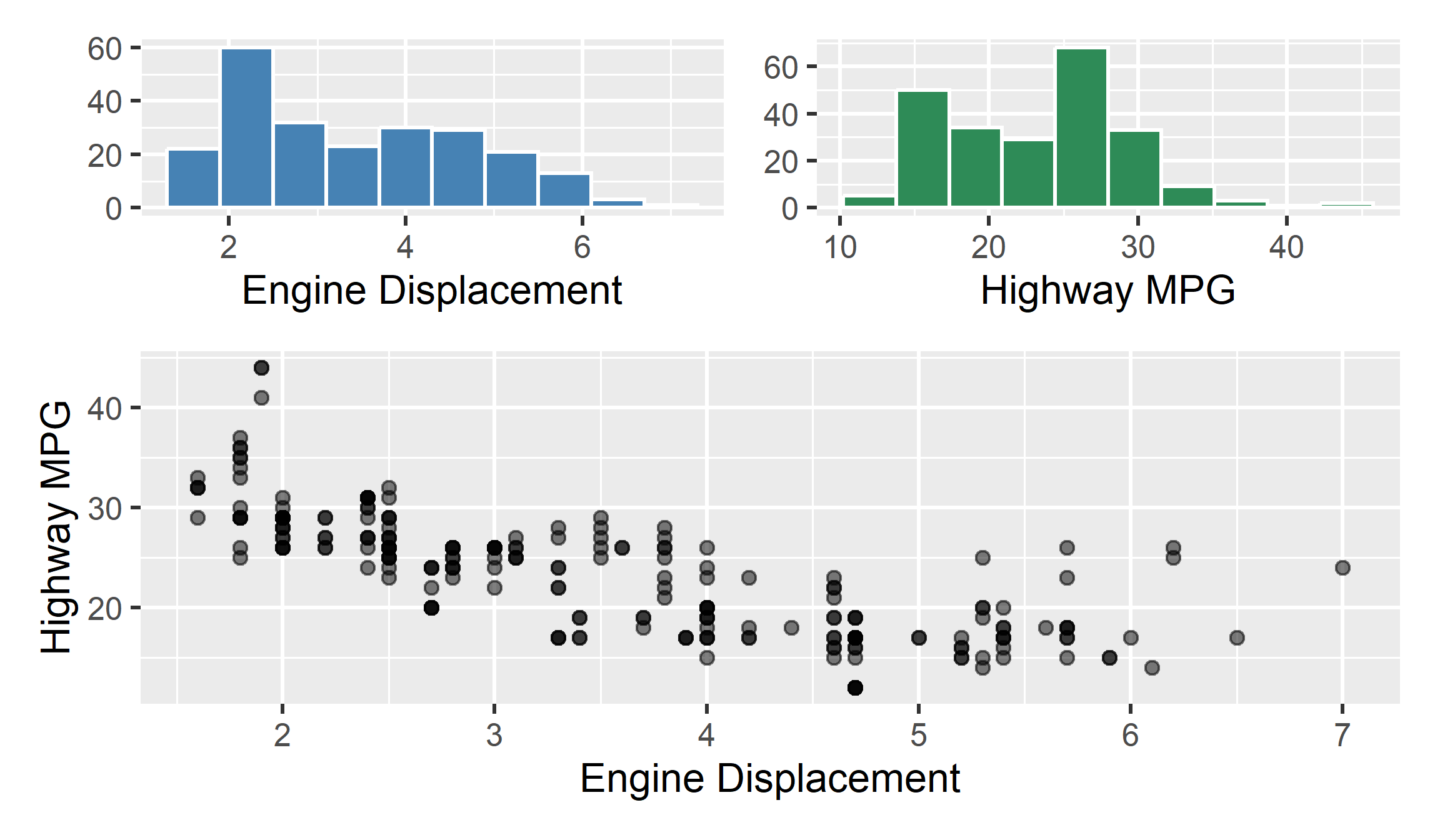
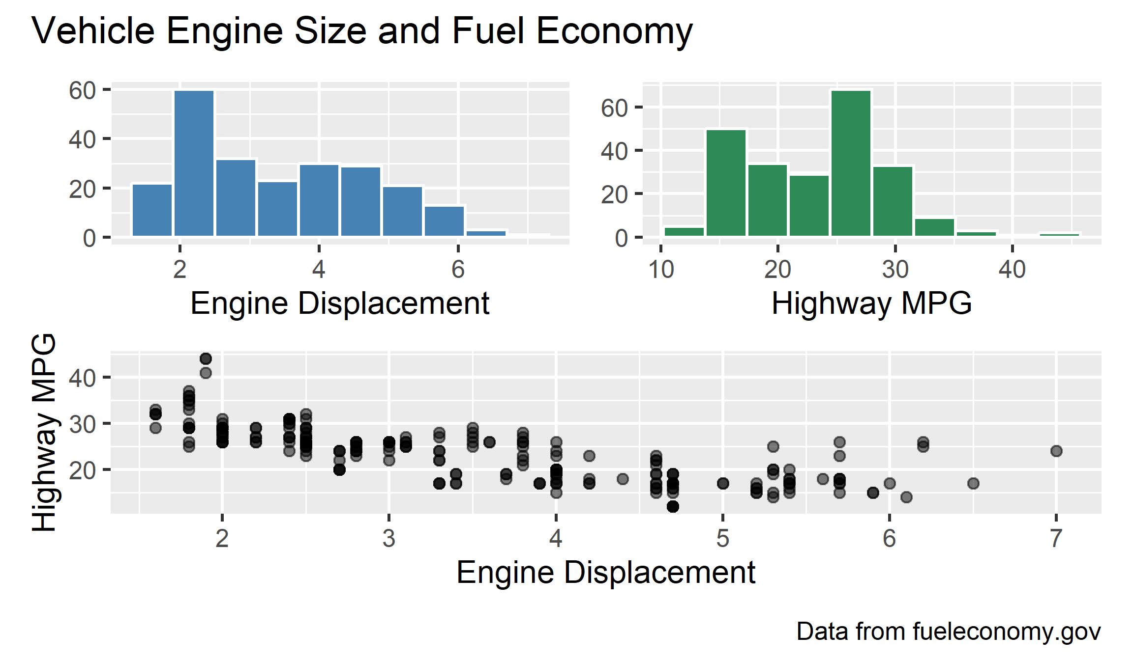
Overall Annotations
# plot_annotation() adds a master title, subtitle, or caption
(p1 | p2) / p3 +
  plot_annotation(
    title = "Vehicle Engine Size and Fuel Economy",
    caption = "Data from fueleconomy.gov"
  )
Automated Tagging
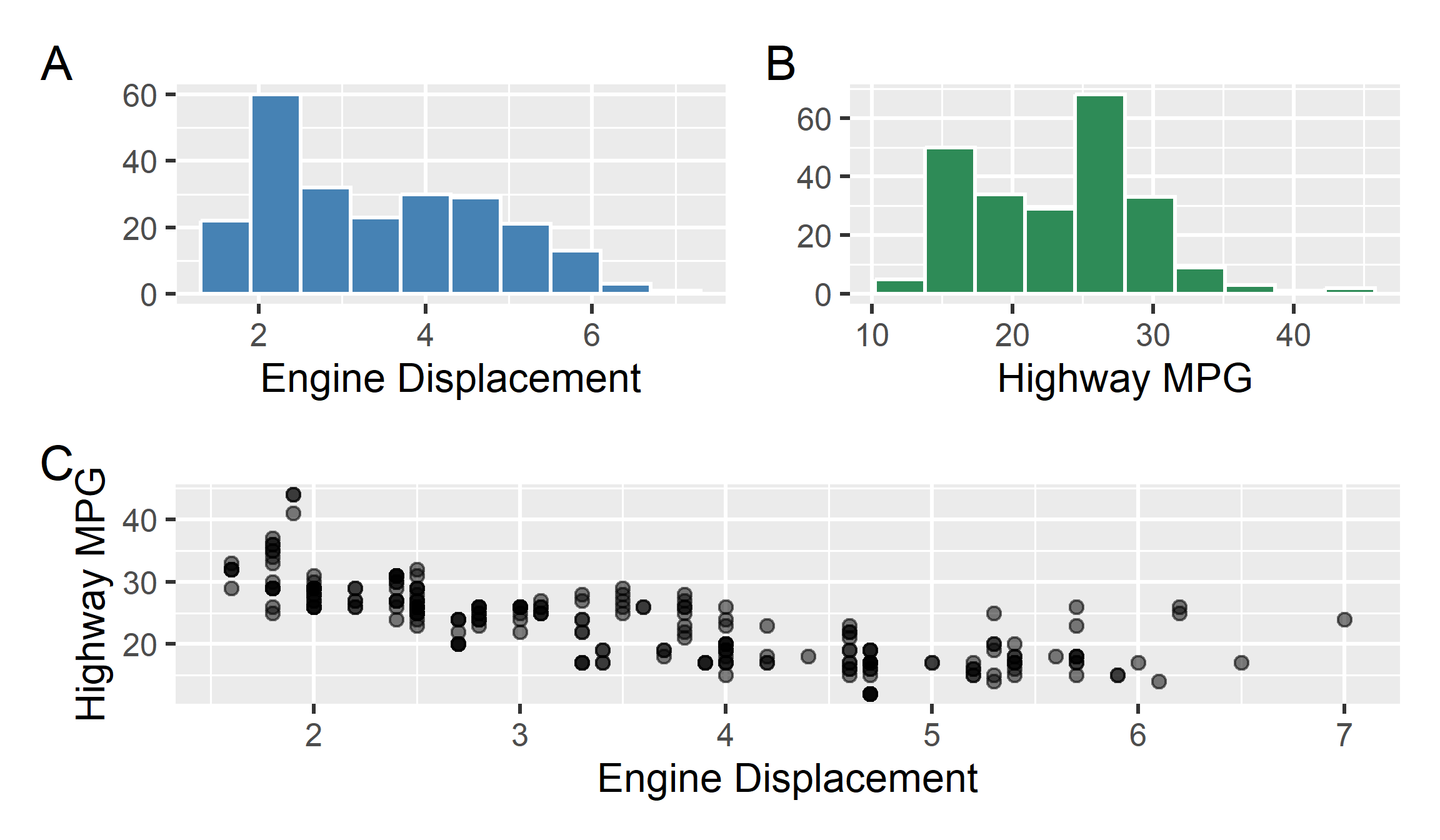
# tag_levels automatically labels subfigures (e.g., A, B, C or 1, 2, 3)
(p1 | p2) / p3 +
  plot_annotation(tag_levels = "A")