Foundations of
Data Science

Spring 2026 | Data 2 (399)
Jeffrey M. Girard | Lecture 14b

Roadmap

Package repetitive code into custom functions using the DRY principle
Control function behavior using arguments, defaults, and branching logic
Apply custom vector functions inside tidyverse data pipelines

Why Write Functions?

The DRY Principle

As you code, you may find yourself copying and pasting code over and over.
This violates the DRY Principle:
“Don’t Repeat Yourself!”
Repetition increases the chance of errors and makes your code harder to read.
Functions allow us to package code into reusable (and sharable) tools.

Repetitive Code Example

library(tidyverse)
data("mpg", package = "ggplot2")
data("starwars", package = "dplyr")

# We want quick histograms to explore our data
p1 <- ggplot(mpg, aes(x = hwy)) + geom_histogram()
p2 <- ggplot(mpg, aes(x = cty)) + geom_histogram()
p3 <- ggplot(starwars, aes(x = height)) + geom_histogram()

This is a lot of typing just to look at three distributions!

Could we make a function to do this more efficiently?

Anatomy of a Function

How Functions Work

A function declaration always requires four core parts:

Name: How we will call the function later.
Arguments: The inputs the function expects.
Body: The actual code that does the work.
(This can be ANY valid R code, e.g., wrangling, visualizing, modeling)
Return: The final output given back to the user.

function_name <- function(arguments) { 
  # function_body
  # ...
  # return_value
}

Our First Function

Let’s build a function to automate our histogram plotting.
It will take a single vector of numbers and return a plot.

gghist <- function(vector) {
  
  # 1. Put the vector into a dataframe
  df <- tibble(x = vector)
  
  # 2. Build the plot
  p <- ggplot(df, aes(x = x)) + geom_histogram()
  
  # 3. Return the plot
  p
}

Using Our Function

Now we can generate our plots with less typing!

gghist(mpg$hwy)

gghist(starwars$height)

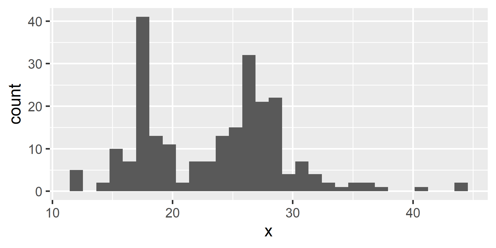
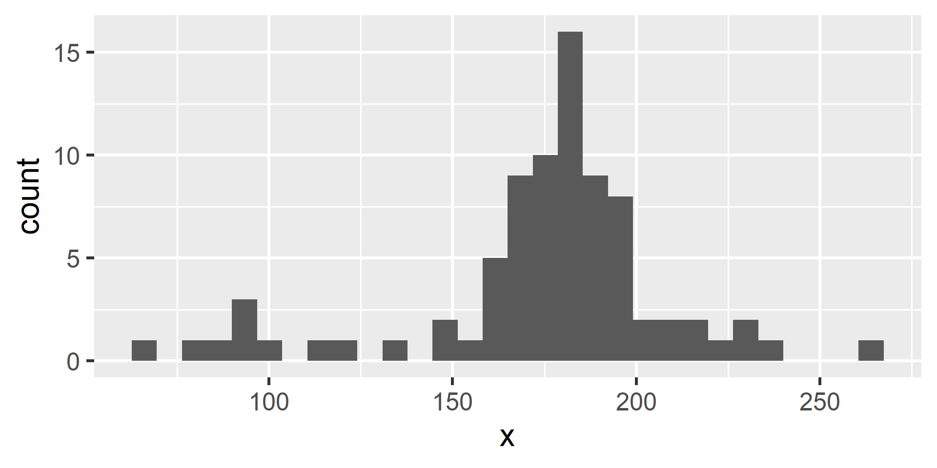
Arguments & Defaults

Adding More Arguments

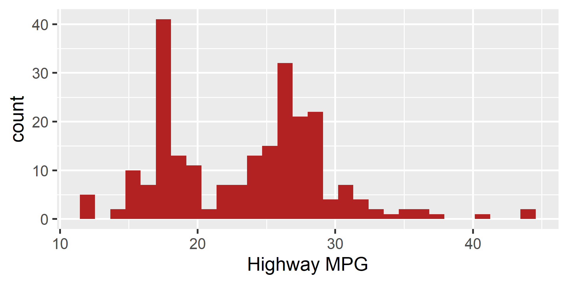
What if we want to change the fill color of our histogram or the text of our
x-axis label? We can simply add more arguments and use them in the body.

gghist_color <- function(vector, fcolor, xlabel) {
  
  df <- tibble(x = vector)
  
  p <- ggplot(df, aes(x = x)) + 
    geom_histogram(fill = fcolor) +
    labs(x = xlabel)
  
  p
}

Using the Arguments

gghist_color(mpg$hwy, fcolor = "firebrick", xlabel = "Highway MPG")

The Missing Argument Error

If we use our new function but forget to provide the new arguments, R will throw an error because it doesn’t know what color/label to use.

gghist_color(mpg$hwy)

Error in `gghist_color()`:
! argument "fcolor" is missing, with no default

We can fix this by setting default argument values.

Setting Defaults

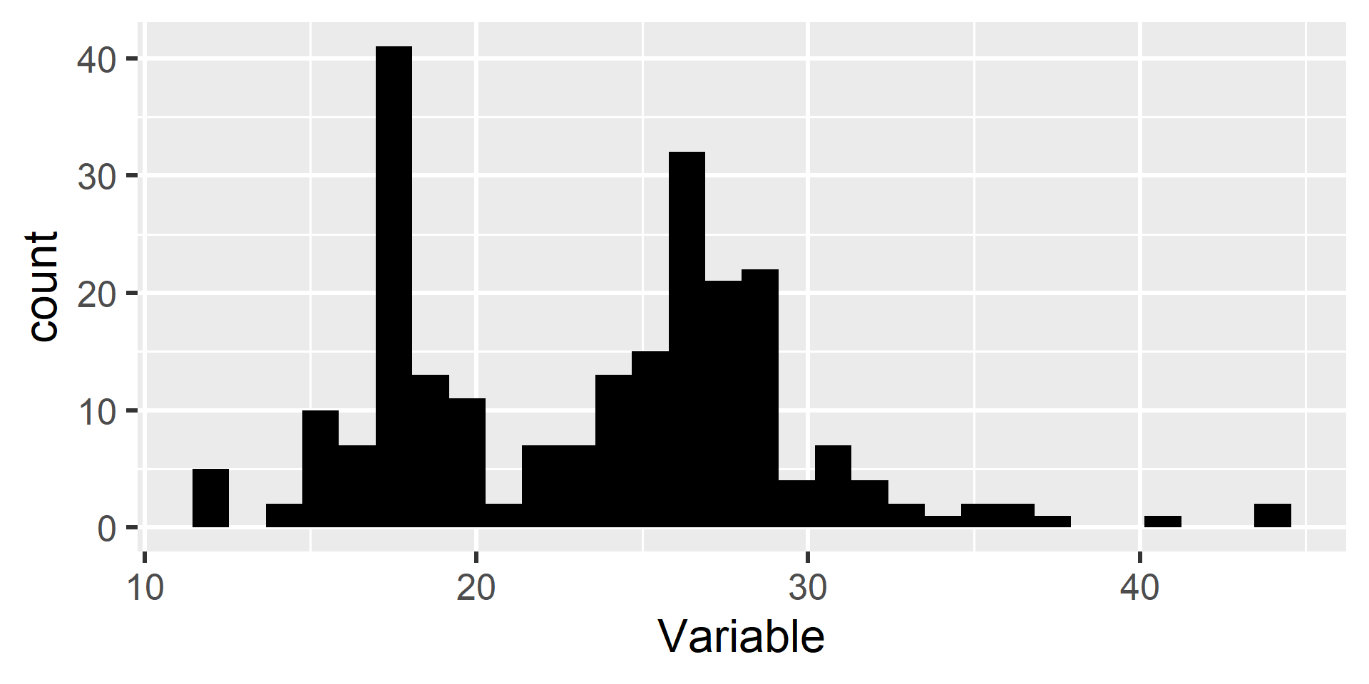
We define defaults in the function() declaration. The default will only be used if the argument is missing. The user can still overwrite the defaults!

gghist_safe <- function(vector, fcolor = "black", xlabel = "Variable") {
  
  df <- tibble(x = vector)
  
  p <- ggplot(df, aes(x = x)) + 
    geom_histogram(fill = fcolor) +
    labs(x = xlabel)
  
  p
}

Using the Defaults

# Provide neither arg
gghist_safe(mpg$hwy)

# Provide one only arg
gghist_safe(mpg$hwy, fcolor = "blue")

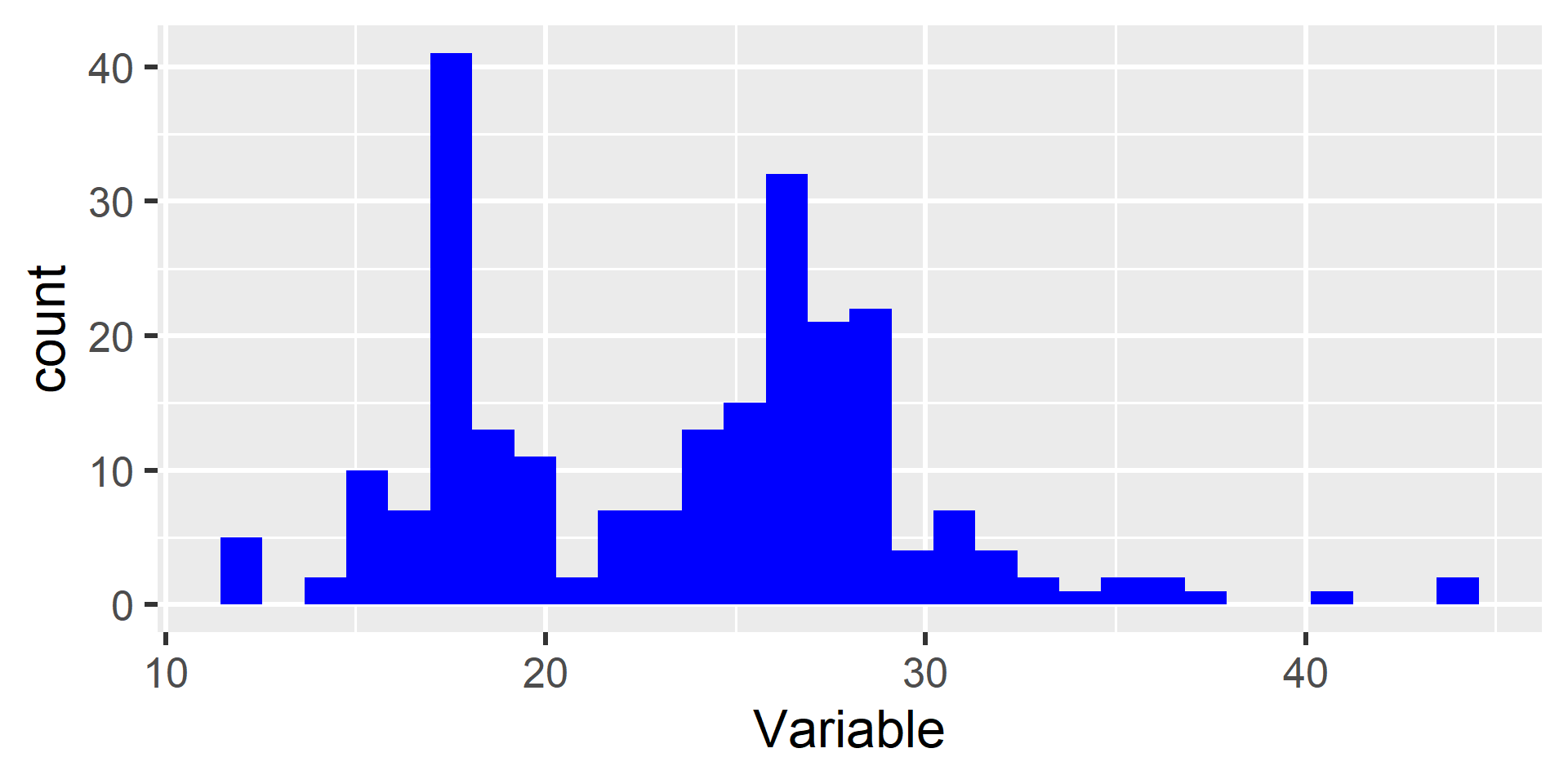
Validation and
Control Flow

Designing for Safety

When sharing functions, the user may not provide the correct data type.
Let’s make a simple function to “center” a variable by subtracting its mean.

center_var <- function(x) {
  x - mean(x, na.rm = TRUE)
}
center_var(c(8, 10, 12))

[1] -2  0  2

center_var(c("apple", "banana", "cherry"))

Error in `x - mean(x, na.rm = TRUE)`:
! non-numeric argument to binary operator

Our function gives an error message, but it is not a very helpful one…

Luckily, we can modify our function to do better!

Input Validation

We can use an if() statement at the very beginning of our function to check the input. If the input is wrong, we use stop() to print an error message.

center_var_safe <- function(x) {
  
  if (!is.numeric(x)) {
    stop("The input vector 'x' must be numeric.")
  }
  
  x - mean(x, na.rm = TRUE)
}

center_var_safe(c("apple", "banana", "cherry"))

Error in `center_var_safe()`:
! The input vector 'x' must be numeric.

Adding Logical Controls

We can add logical arguments (TRUE or FALSE) to give users control over how the function operates. Let’s add a robust argument to our centering function.

center_var_adv <- function(x, robust = FALSE) {
  
  if (!is.numeric(x)) { stop("Input 'x' must be numeric.") }
  if (!is.logical(robust)) { stop("Input 'robust' must be logical.")}
  
  # But how do we use the robust argument?
  # - we want to subtract the mean if robust is FALSE (default)
  # - we want to subtract the median if robust is TRUE
}

Branching Logic

We can use an if and else block to create two branches in our function.
The code will do different things based on the robust argument’s value.

center_var_adv <- function(x, robust = FALSE) {
  
  if (!is.numeric(x)) { stop("Input 'x' must be numeric.") }
  if (!is.logical(robust)) { stop("Input 'robust' must be logical.")}
  
  if (robust == TRUE) {
    # The robust branch uses the median
    centered <- x - median(x, na.rm = TRUE)
  } else {
    # The standard branch uses the mean
    centered <- x - mean(x, na.rm = TRUE)
  }
  
  centered
}

Using the Branching Function

Because the mean is highly sensitive to outliers, our robust argument provides a very helpful alternative path!

my_data <- c(1, 2, 3, 4, 100) # Notice the outlier

# Standard centering is greatly influenced by the outlier
center_var_adv(my_data, robust = FALSE)

[1] -21 -20 -19 -18  78

# Robust centering is not influenced by the outlier
center_var_adv(my_data, robust = TRUE)

[1] -2 -1  0  1 97

Functions in Pipelines

The Payoff in mutate()

Because our center_var_adv() function takes a vector and returns a vector of the same length, it drops perfectly into our tidyverse pipelines.

mpg |> 
  select(manufacturer, model, hwy) |> 
  mutate(
    hwy_cent = center_var_adv(hwy),
    hwy_rob = center_var_adv(hwy, robust = TRUE)
  )

# A tibble: 234 × 5
  manufacturer model   hwy hwy_cent hwy_rob
  <chr>        <chr> <int>    <dbl>   <dbl>
1 audi         a4       29     5.56       5
2 audi         a4       29     5.56       5
3 audi         a4       31     7.56       7
4 audi         a4       30     6.56       6
5 audi         a4       26     2.56       2
# ℹ 229 more rows

Prepping for Iteration

You can build any mathematical transformation you need and apply it the same way. For example, a common task is standardization (z-scoring):

standardize <- function(x) {
  (x - mean(x, na.rm = TRUE)) / sd(x, na.rm = TRUE)
}
mpg |> 
  select(manufacturer, model, cty) |> 
  mutate(cty_z = standardize(cty))

# A tibble: 234 × 4
  manufacturer model   cty  cty_z
  <chr>        <chr> <int>  <dbl>
1 audi         a4       18  0.268
2 audi         a4       21  0.973
3 audi         a4       20  0.738
4 audi         a4       21  0.973
5 audi         a4       16 -0.202
# ℹ 229 more rows

Summary

Limitless Potential: Functions can package any valid R code or workflow.
Reduce Repetition: They apply the DRY principle.
Structure: They require a name, arguments, a body, and a return value.
Arguments & Logic: You can set default values and use if/else to branch function behavior.
Validation: Use if() and stop() to ensure the correct data is provided.
Functions in Pipelines: Custom functions that return vectors drop seamlessly into mutate() and prepare us for iteration.

Foundations of Data Science