Foundations of
Data Science

Spring 2026 | Data 2 (399)
Jeffrey M. Girard | Lecture 14c

Roadmap

Iterate functions across multiple columns using across()
Use list objects to store complex, mixed-type data
Efficiently apply functions to vectors using map()

Iterating Over Columns

The Repetition Problem

We often need to apply the exact same function to many different columns. Doing this manually requires a lot of repetitive, error-prone typing.

library(tidyverse)
data("mpg", package = "ggplot2")

# Calculating the mean for multiple columns manually
mpg |> 
  summarize(
    cty_mean = mean(cty),
    hwy_mean = mean(hwy),
    displ_mean = mean(displ)
  )

# A tibble: 1 × 3
  cty_mean hwy_mean displ_mean
     <dbl>    <dbl>      <dbl>
1     16.9     23.4       3.47

Introducing across()

The across() function solves this by allowing us to apply the same transformation to multiple columns simultaneously. It takes two primary arguments: .cols (which columns) and .fns (what function).

# This does the exact same thing, but much more efficiently
mpg |> 
  summarize(
    across(.cols = c(cty, hwy, displ), .fns = mean)
  )

# A tibble: 1 × 3
    cty   hwy displ
  <dbl> <dbl> <dbl>
1  16.9  23.4  3.47

Selecting Columns Smartly

We can use tidy-select helpers (like where(), starts_with(), or contains()) inside of across() to target specific types of columns.

# Apply the mean function to all numeric columns at once
mpg |> 
  summarize(
    across(.cols = where(is.numeric), .fns = mean)
  )

# A tibble: 1 × 5
  displ  year   cyl   cty   hwy
  <dbl> <dbl> <dbl> <dbl> <dbl>
1  3.47 2004.  5.89  16.9  23.4

Custom Functions Work Too

Importantly, across() works perfectly with custom functions! It also drops right into mutate() just as easily as summarize().

# Our standardization function from Lecture 14b
standardize <- function(x) { (x - mean(x, na.rm = TRUE)) / sd(x, na.rm = TRUE) }

mpg |> 
  mutate(across(.cols = c(cty, hwy), .fns = standardize)) |> 
  select(manufacturer, cty, hwy)

# A tibble: 234 × 3
  manufacturer    cty   hwy
  <chr>         <dbl> <dbl>
1 audi          0.268 0.934
2 audi          0.973 0.934
3 audi          0.738 1.27 
4 audi          0.973 1.10 
5 audi         -0.202 0.430
# ℹ 229 more rows

Anonymous Functions

The Need for Quick Functions

Sometimes we need to apply a simple operation across many columns, but it feels overkill to create and save a custom, named function for it.

# Do we really need to save this just to use it once?
multiply_by_ten <- function(x) { x * 10 }

mpg |> 
  mutate(across(c(cty, hwy), multiply_by_ten)) |> 
  select(manufacturer, cty, hwy)

# A tibble: 234 × 3
  manufacturer   cty   hwy
  <chr>        <dbl> <dbl>
1 audi           180   290
2 audi           210   290
3 audi           200   310
4 audi           210   300
5 audi           160   260
# ℹ 229 more rows

The (x) Syntax

R allows us to write anonymous functions (functions without a name) directly inside our pipelines using the \(x) syntax. This simply tells R: “I am about to write a temporary function that takes a single argument that we can call x.”

# This code does the exact same thing, but inline!
mpg |> 
  mutate(across(c(cty, hwy), \(x) x * 10)) |> 
  select(manufacturer, cty, hwy)

# A tibble: 234 × 3
  manufacturer   cty   hwy
  <chr>        <dbl> <dbl>
1 audi           180   290
2 audi           210   290
3 audi           200   310
4 audi           210   300
5 audi           160   260
# ℹ 229 more rows

Passing Arguments

One of the biggest advantage of anonymous functions is how easily they let us pass additional arguments to the function we are iterating (e.g., na.rm).

# How to pass na.rm = TRUE to mean()?
starwars |> 
  summarize(
    across(
      .cols = c(mass, height), 
      .fns = mean
    )
  )

# A tibble: 1 × 2
   mass height
  <dbl>  <dbl>
1    NA     NA

# With an anonymous function!
starwars |> 
  summarize(
    across(
      .cols = c(mass, height), 
      .fns = \(x) mean(x, na.rm = TRUE)
    )
  )

# A tibble: 1 × 2
   mass height
  <dbl>  <dbl>
1  97.3   175.

Understanding Lists

The Limits of Standard Vectors

We know how to store data in standard, atomic vectors using c().
The limitation: Every item in a vector must be the same data type.
- If you mix multiple types, c() converts them to be the same.
The solution: A list is a special “super vector” that can hold anything.

# logicals < *numbers* < characters
c(0, 1, 0, TRUE, FALSE)

[1] 0 1 0 1 0

# logicals < numbers < *characters*
c(42.1, "Hello World", TRUE)

[1] "42.1"        "Hello World" "TRUE"

list(42.1, "Hello World", TRUE)

[[1]]
[1] 42.1

[[2]]
[1] "Hello World"

[[3]]
[1] TRUE

Lists Can Store Anything

wow <- list(
  tibble(x = 1:2, y = c("a", "b")),
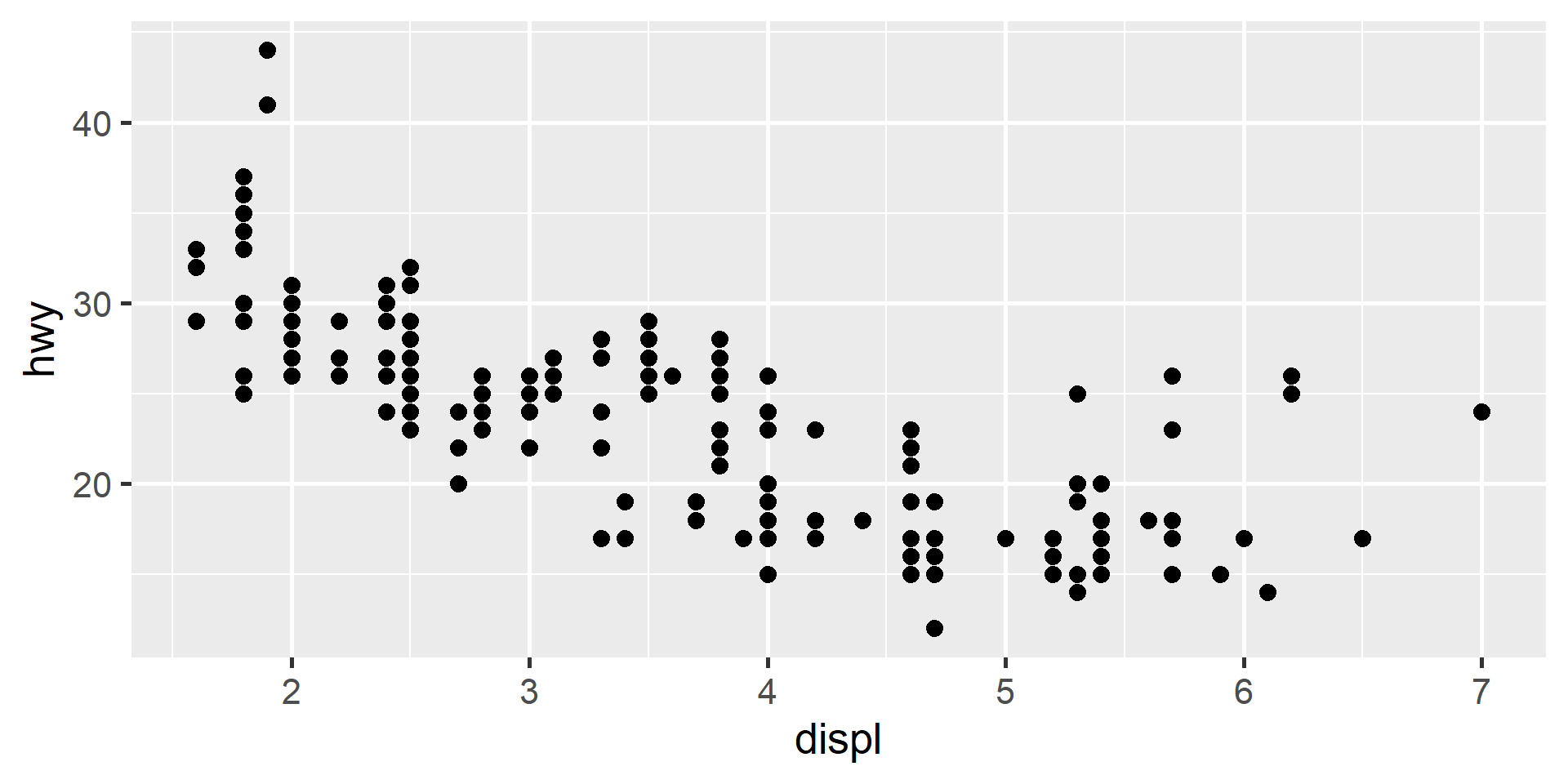
  ggplot(mpg, aes(x = displ, y = hwy)) + geom_point()
)

wow[[1]]

# A tibble: 2 × 2
      x y    
  <int> <chr>
1     1 a    
2     2 b

wow[[2]]

Naming List Elements

# Set names during creation
my_list <- 
  list(
    myNumbers = c(1, 2, 3),
    myLetters = c("x", "y")
  ) |> 
  print()

$myNumbers
[1] 1 2 3

$myLetters
[1] "x" "y"

# Set names after creation
my_list <- 
  list(
    c(1, 2, 3),
    c("x", "y")
  ) |> 
  set_names(
    c("myNumbers", "myLetters")
  ) |> 
  print()

$myNumbers
[1] 1 2 3

$myLetters
[1] "x" "y"

Iterating Over Vectors

Two Ways to Iterate

We use across() to iterate over columns, but what about vectors?
The Traditional Approach: Loops
- Many programmers use loops to manually micro-manage iteration (e.g., creating empty containers, filling them, and tracking exact positions).
The Tidyverse Approach: {purrr}
- We will use functional programming to “delegate” the boring work
- Simplicity: Provide just the vector and the function.
- Automation: Automatically tracks positions and stores results.
- Readability: Integrates cleanly into pipelines.

How map() Works

The core function map() takes a vector (.x) and a function (.f)
Toy Example: Generating samples of different sizes
- runif(n) generates n random numbers between 0 and 1

# Generate a sample of random numbers for each sample size
my_samples <- map(.x = c(2, 4, 3), .f = runif)
my_samples

[[1]]
[1] 0.08239532 0.35262510

[[2]]
[1] 0.6659183 0.5287297 0.3844625 0.8534727

[[3]]
[1] 0.9886961 0.8799051 0.1221085

Type-Specific Maps

If the output is all one type, we can simplify it with a type-specific map
- e.g., map_dbl() returns a numeric vector
- e.g., map_chr() returns a character vector
Example: Finding the maximum value in each of our random samples

# Keep output as a list
map(.x = my_samples, .f = max)

[[1]]
[1] 0.3526251

[[2]]
[1] 0.8534727

[[3]]
[1] 0.9886961

# Simplify to a numeric vector
map_dbl(.x = my_samples, .f = max)

[1] 0.3526251 0.8534727 0.9886961

Step 1: Finding Our Files

The real power of map() is working with complex data structures like files.
The Scenario: You have a folder full of CSV files to combine.
First, we need to locate them using list.files()
- path: Which folder to look in
- pattern: What regex pattern to look for (ends in “.csv”)
- full.names: Keep this TRUE so R knows exactly where the file is

# This outputs a simple character vector of file paths
my_files <- list.files(path = "data", pattern = "\\.csv$", full.names = TRUE)
my_files

[1] "data/pid_001.csv" "data/pid_002.csv" "data/pid_003.csv"

Step 2: Reading Files into a List

Now we have a character vector of file paths.
We can use map() to apply the read_csv() function to every path.
Since map() always returns a list, we will get a list where each item is a complete data frame.

list_of_dfs <- 
  # read each file as a tibble into a list object
  map(.x = my_files, .f = read_csv) |> 
  # set the name of each element to be its file path
  set_names(my_files)

Previewing the List

list_of_dfs

$`data/pid_001.csv`
# A tibble: 30 × 2
    day  mood
  <dbl> <dbl>
1     1     5
2     2     4
3     3     3
4     4     5
5     5     4
# ℹ 25 more rows

$`data/pid_002.csv`
# A tibble: 30 × 2
    day  mood
  <dbl> <dbl>
1     1     4
2     2     5
3     3     3
4     4     4
5     5     3
# ℹ 25 more rows

$`data/pid_003.csv`
# A tibble: 30 × 2
    day  mood
  <dbl> <dbl>
1     1     6
2     2     3
3     3     0
4     4     2
5     5     6
# ℹ 25 more rows

Step 3: Binding the Data

We have our data, but a list of data frames is difficult to analyze
We want one combined data frame
list_rbind() will stacks them row-by-row
- The names_to argument creates a helpful ID column so we know where each row came from.

alldata <- list_rbind(list_of_dfs, names_to = "file")

Previewing the Combined Data

# One 90-row tibble instead of three 30-row tibbles
alldata

# A tibble: 90 × 3
  file               day  mood
  <chr>            <dbl> <dbl>
1 data/pid_001.csv     1     5
2 data/pid_001.csv     2     4
3 data/pid_001.csv     3     3
4 data/pid_001.csv     4     5
5 data/pid_001.csv     5     4
# ℹ 85 more rows

Using the Combined Data

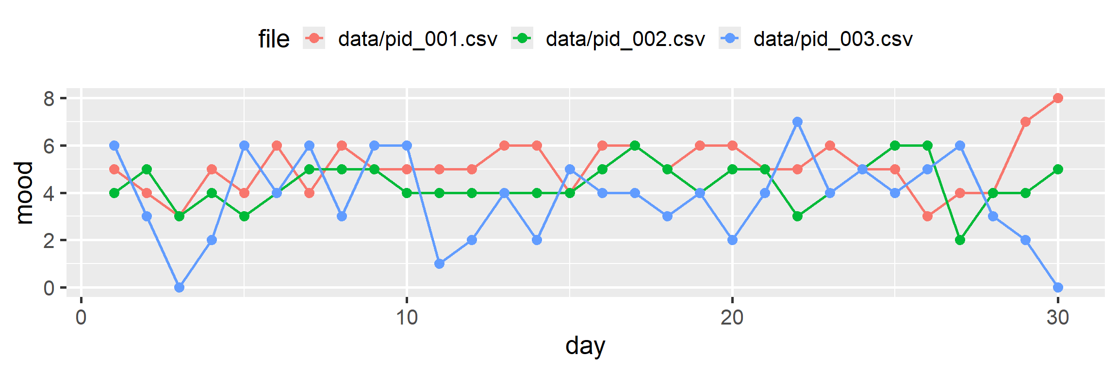
alldata |> 
  ggplot(aes(x = day, y = mood, color = file, group = file)) +
  geom_line() + geom_point() +
  theme(legend.position = "top")

Iterating for Side Effects

# Create function to read in data, create a plot, and save it
create_plot <- function(file) {
  # Read in the data from current file
  current_data <- read_csv(file)
  # Create plot of the current data
  current_plot <- ggplot(current_data, aes(x = day, y = mood)) +
    geom_line() + geom_point() + labs(title = file)
  # Save the plot to a png image file
  ggsave(filename = str_glue("{file}.png"), plot = current_plot,
    width = 7, height = 5, units = "in")
  # Return the plot object
  current_plot
}

# Apply this function to each of my_files
p <- map(.x = my_files, .f = create_plot)

Verifying it worked

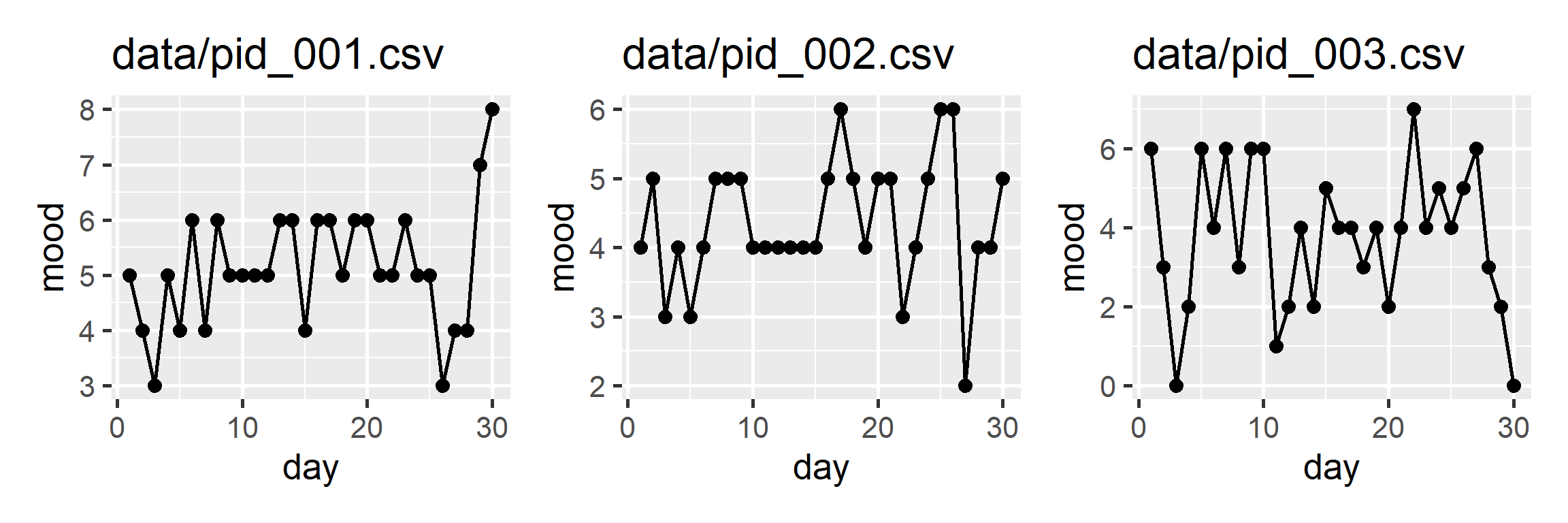
library(patchwork)
p[[1]] + p[[2]] + p[[3]]

list.files(path = "data", pattern = "\\.png$", full.names = TRUE)

[1] "data/pid_001.csv.png" "data/pid_002.csv.png" "data/pid_003.csv.png"

Foundations of Data Science