Sample Demographics

library(tidyverse)
library(datawizard)
library(kableExtra)

# Sessions and human MADRS totals (NDA madrs01), and participant
# characteristics (NDA ndar_subject01)
source("load_data.R")
obs_raw <- load_prediction_sheets(conditions = "full")[[1]]
demo_raw <- load_subjects()

Session Summaries

obs_tidy <- 
  obs_raw |> 
  select(
    patient, 
    session,
    visit_no,
    madrs = ground_truth
  ) |> 
  summarize(
    .by = c(patient, session, visit_no),
    madrs = first(madrs)
  )

obs_tidy |> 
  describe_distribution(select = "madrs") |> 
  print_md()

Variable	Mean	SD	IQR	Range	Skewness	Kurtosis	n	n_Missing
madrs	20.19	11.90	19	(0.00, 54.00)	0.28	-0.73	541	0

obs_tidy |> 
  summarize(.by = patient, n_sessions = n()) |> 
  describe_distribution(select = "n_sessions") |> 
  print_md()

Variable	Mean	SD	IQR	Range	Skewness	Kurtosis	n	n_Missing
n_sessions	1.95	1.25	1	(1.00, 8.00)	1.72	3.41	277	0

ggplot(obs_tidy, aes(x = visit_no)) + 
  geom_bar() +
  scale_x_continuous(breaks = 1:8) +
  labs(x = "Visit Number", y = "Number of Sessions") +
  theme_bw(base_size = 10)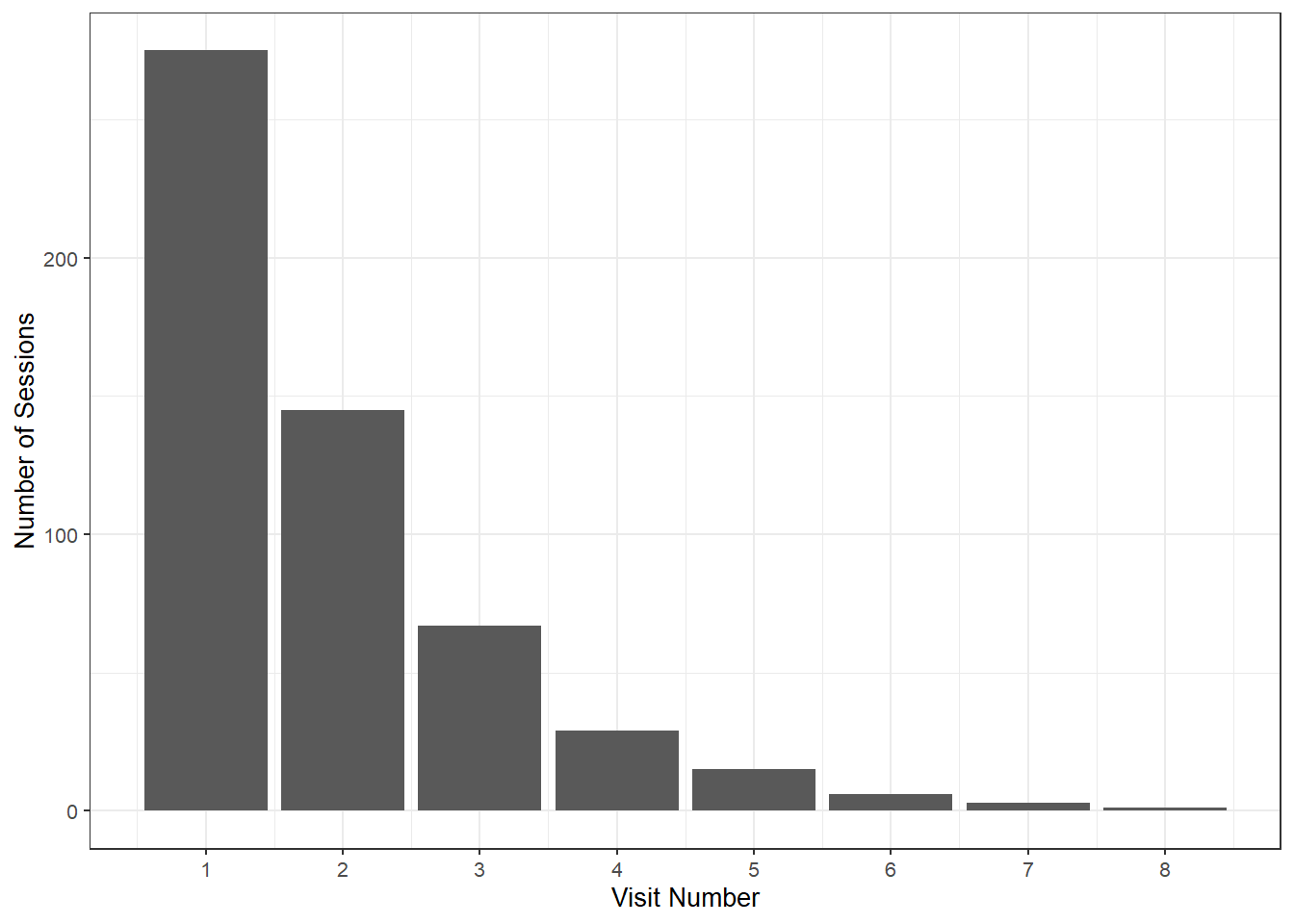

bin_width <- 5
n_obs <- nrow(obs_tidy)

ggplot(obs_tidy, aes(x = madrs)) + 
  geom_histogram(
    breaks = seq(0, 60, bin_width), 
    color = "black",
    fill  = "grey80"
  ) +
  geom_density(
    aes(y = after_stat(density * n_obs * bin_width)),
    color    = "blue",
    linewidth = 1
  ) +
  labs(
    x = "MADRS Total Score",
    y = "Number of Sessions"
  ) +
  theme_bw(base_size = 10)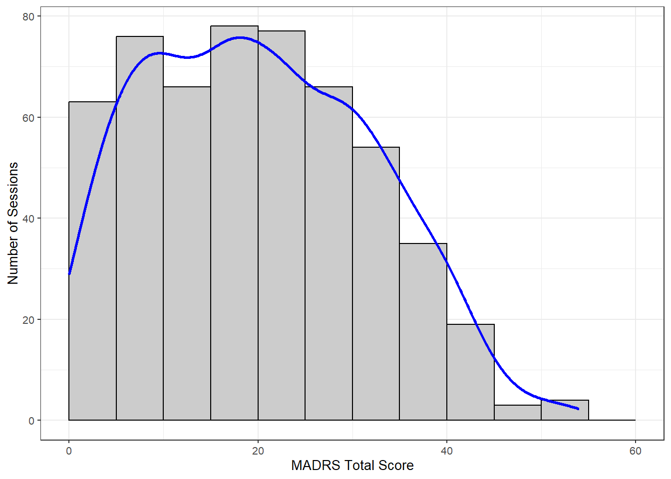

Patient Summaries

demo_tidy <- 
  demo_raw |> 
  transmute(
    patient,
    diagnosis = fct_collapse(
      diagnosis,
      bipolar = c("BP1 (depressed)", "BP1 (hypomanic)", "BP1 (manic)", "BP1 (mixed)", "BP2 (depressed)", "BP2 (hypomanic)", "BP NOS"),
      major_depressive = c("MDD", "MDD w/ psychosis"),
      schizophrenia = "SZ",
      schizoaffective = c("SZA (bp)", "SZA (dep)"),
      psychosis_nos = "Psychosis NOS",
      other = "Other"
    ),
    sex = factor(sex),
    race = fct_lump_prop(
      race,
      prop = 0.01
    ),
    ethnicity = factor(ethnicity),
    education = fct_na_value_to_level(
      education,
      level = "Prefer not to answer/Unknown"
    ),
    age
  ) |>
  filter(patient %in% unique(obs_tidy$patient)) |> 
  mutate(patient = factor(patient)) |> 
  summarize(
    .by = patient,
    across(everything(), first)
  )

demo_tidy |> 
  describe_distribution(select = "age") |> 
  print_md()

Variable	Mean	SD	IQR	Range	Skewness	Kurtosis	n	n_Missing
age	39.78	14.34	26.50	(18.00, 74.00)	0.18	-1.22	277	0

demo_tidy |> 
  data_tabulate(
    select = c("sex", "race", "ethnicity", "education", "diagnosis")
  ) |> 
  print_md()

Frequency Table

Variable	Value	N	Raw %	Valid %	Cumulative %
sex	Female	120	43.32	43.32	43.32
	Male	157	56.68	56.68	100.00
	NR	0	0.00	0.00	100.00
	(NA)	0	0.00	(NA)	(NA)
race	Asian	10	3.61	3.61	3.61
	Black or African American	32	11.55	11.55	15.16
	More than one race	5	1.81	1.81	16.97
	White	208	75.09	75.09	92.06
	Other	22	7.94	7.94	100.00
	(NA)	0	0.00	(NA)	(NA)
ethnicity	Hispanic or Latino	36	13.00	13.00	13.00
	Not Hispanic or Latino	234	84.48	84.48	97.47
	Unknown or not reported	7	2.53	2.53	100.00
	(NA)	0	0.00	(NA)	(NA)
education	Less than High School	16	5.78	5.78	5.78
	High School/GED	57	20.58	20.58	26.35
	Part College or 2-year degree	103	37.18	37.18	63.54
	4-year College degree	50	18.05	18.05	81.59
	Part or completed Graduate degree	33	11.91	11.91	93.50
	Prefer not to answer/Unknown	18	6.50	6.50	100.00
	(NA)	0	0.00	(NA)	(NA)
diagnosis	bipolar	85	30.69	30.69	30.69
	major_depressive	96	34.66	34.66	65.34
	other	13	4.69	4.69	70.04
	psychosis_nos	20	7.22	7.22	77.26
	schizophrenia	17	6.14	6.14	83.39
	schizoaffective	46	16.61	16.61	100.00
	(NA)	0	0.00	(NA)	(NA)