Performance Analyses

Setup

library(tidyverse)
library(patchwork)
library(furrr)
library(gt)

plan("multisession", workers = 10)

Tidy Data

# Predictions (public, ../data) joined to human ratings (NDA, ../nda)
source("load_data.R")
fewshot_raw <- load_prediction_sheets(conditions = "full")
fewshot_sheets <- names(fewshot_raw)

# Sessions used as fewshot examples (excluded from evaluation)
excluded_ids <- load_exemplars()

# Collect total score labels and direct total score predictions 
fewshot_total <- 
  fewshot_raw[[1]] |> 
  select(
    session, patient, model_name,
    ground_truth, rating_0, rating_1, rating_2
  ) |> 
  filter(session %in% excluded_ids[[1]] == FALSE) |> 
  summarize(
    .by = c(session, patient, model_name),
    label00 = mean(ground_truth) / 10,
    direct00 = rowMeans(pick(rating_0, rating_1, rating_2), na.rm = TRUE) / 10
  )

# Collect item score labels and item score predictions
item_indices <- 2:11

item_dfs <- map(
  item_indices,
  \(i) {
    gt_name <- sprintf("label%02d", i-1)
    pv_name <- sprintf("pred%02d", i-1)
    fewshot_raw[[i]] |>
      transmute(
        session,
        patient,
        model_name,
        !!gt_name := ground_truth,
        !!pv_name := rowMeans(pick(rating_0, rating_1, rating_2), na.rm = TRUE)
      ) |> 
      filter(session %in% excluded_ids[[i]] == FALSE)
  }
)

# Combine collected data and calculate indirect total score predictions
fewshot_all <- 
  reduce(
    item_dfs, 
    ~ full_join(.x, .y, by = c("session", "patient", "model_name"))
  ) |> 
  mutate(
    indirect00 = rowMeans(
      pick(num_range(prefix = "pred", range = 1:10, width = 2)), 
      na.rm = FALSE
    )
  ) |> 
  full_join(fewshot_total, by = c("session", "patient", "model_name")) |> 
  relocate(label00, .before = indirect00)

Setup and Run Cluster Bootstrap Analysis

cluster_boot_comparison <- function(
  dat,
  B    = 10000,
  seed = 2026
){
  # --------------------------------------------------------------------------
  # Helpers ------------------------------------------------------------------
  # --------------------------------------------------------------------------
  ccc_vec <- \(x, y) {
    ok <- complete.cases(x, y)
    x  <- x[ok]
    y  <- y[ok]

    # guard against tiny samples / no variance
    if (length(x) < 2L) return(NA_real_)
    var_x <- var(x)
    var_y <- var(y)
    if (var_x == 0 || var_y == 0) return(NA_real_)

    mu_x   <- mean(x)
    mu_y   <- mean(y)
    cov_xy <- cov(x, y)
    (2 * cov_xy) / (var_x + var_y + (mu_x - mu_y)^2)
  }

  calc_null_shifted_pvalue <- function(boot_dist, obs_val) {
    boot_dist <- boot_dist[!is.na(boot_dist)]
    if(length(boot_dist) == 0) return(NA_real_)
    null_dist <- boot_dist - mean(boot_dist)
    mean(abs(null_dist) >= abs(obs_val))
  }

  # --------------------------------------------------------------------------
  # Pre-split by patient (cluster bootstrap units) ---------------------------
  # --------------------------------------------------------------------------
  patient_list <- dat |> group_split(patient, .keep = TRUE)
  n_patients   <- length(patient_list)

  # --------------------------------------------------------------------------
  # Pre-pivot and Pre-split Data ---------------------------------------------
  # --------------------------------------------------------------------------
  items_long <-
    dat |>
    pivot_longer(
      cols = matches("^(label|pred)(0[1-9]|10)$"),
      names_to = c(".value", "suffix"),
      names_pattern = "(label|pred)(0[1-9]|10)"
    ) |>
    mutate(comparison = paste0("item", suffix)) |>
    select(model_name, patient, comparison, label, pred)

  total_long <-
    dat |>
    select(model_name, patient, label00, direct00, indirect00) |>
    pivot_longer(
      cols = c(direct00, indirect00),
      names_to = "comparison",
      values_to = "pred"
    ) |>
    mutate(
      comparison = if_else(comparison == "direct00", "00_direct", "00_indirect"),
      label = label00
    ) |>
    select(model_name, patient, comparison, label, pred)

  dat_long <- bind_rows(items_long, total_long)
  patient_list <- dat_long |> group_split(patient, .keep = TRUE)
  n_patients <- length(patient_list)

  # --------------------------------------------------------------------------
  # Simplified compute_stats -------------------------------------------------
  # --------------------------------------------------------------------------
  compute_stats <- function(df) {
    df |>
      summarise(
        mae = mean(abs(pred - label), na.rm = TRUE),
        ccc = ccc_vec(pred, label),
        .by = c(model_name, comparison)
      )
  }

  # --------------------------------------------------------------------------
  # Observed (non-bootstrapped) estimates
  # --------------------------------------------------------------------------
  observed <- compute_stats(dat_long)

  # --------------------------------------------------------------------------
  # Bootstrap
  # --------------------------------------------------------------------------
  set.seed(seed)

  boot_results <-
    future_map(
      seq_len(B),
      \(b) {
        idx  <- sample.int(n_patients, size = n_patients, replace = TRUE)
        df_b <- bind_rows(patient_list[idx])
        compute_stats(df_b) |> mutate(boot = b)
      },
      .progress = TRUE,
      .options = furrr_options(
        seed = TRUE, 
        globals = c("patient_list", "compute_stats", "ccc_vec"),
        packages = "dplyr"
      )
    ) |> 
    list_rbind()

  # --------------------------------------------------------------------------
  # Bootstrap CIs for each model × comparison (MAE, CCC)
  # --------------------------------------------------------------------------
  boot_summary <-
    boot_results |>
    summarize(
      mae_lower = quantile(mae, 0.025, na.rm = TRUE),
      mae_upper = quantile(mae, 0.975, na.rm = TRUE),
      ccc_lower = quantile(ccc, 0.025, na.rm = TRUE),
      ccc_upper = quantile(ccc, 0.975, na.rm = TRUE),
      .by = c(model_name, comparison)
    )

  # --------------------------------------------------------------------------
  # Build item01 ... item10 data frames (one per item) -----------------------
  # --------------------------------------------------------------------------
  item_list <- lapply(1:10, function(k) {
    comp <- paste0("item", sprintf("%02d", k))

    obs_k  <- observed |> filter(comparison == comp)
    boot_k <- boot_summary |> filter(comparison == comp)

    obs_k |>
      left_join(boot_k, by = c("model_name", "comparison")) |>
      select(
        model_name,
        mae, mae_lower, mae_upper,
        ccc, ccc_lower, ccc_upper
      )
  })
  names(item_list) <- sprintf("item%02d", 1:10)

  # --------------------------------------------------------------------------
  # Item 00: direct vs indirect, wide + diffs + p-values ---------------------
  # --------------------------------------------------------------------------
  # Observed 00 (long)
  observed00 <-
    observed |>
    filter(comparison %in% c("00_direct", "00_indirect"))

  # Observed 00 (wide): per model, separate cols for direct/indirect
  obs00_wide <-
    observed00 |>
    pivot_wider(
      names_from  = comparison,
      values_from = c(mae, ccc),
      names_glue  = "{.value}_{comparison}"
    )

  # CIs for direct/indirect from bootstrap (still per comparison)
  boot00 <-
    boot_summary |>
    filter(comparison %in% c("00_direct", "00_indirect"))

  # Wide CIs: one row per model, columns for direct & indirect
  boot00_wide <-
    boot00 |>
    pivot_wider(
      names_from  = comparison,
      values_from = c(mae_lower, mae_upper, ccc_lower, ccc_upper),
      names_glue  = "{.value}_{comparison}"
    )

  # Observed differences (indirect - direct)
  observed_diff <-
    obs00_wide |>
    mutate(
      diff_mae_obs = mae_00_indirect - mae_00_direct,
      diff_ccc_obs = ccc_00_indirect - ccc_00_direct
    ) |>
    select(model_name, diff_mae_obs, diff_ccc_obs)

  # Bootstrap differences
  boot_diff <-
    boot_results |>
    filter(comparison %in% c("00_direct", "00_indirect")) |>
    pivot_wider(
      names_from  = comparison,
      values_from = c(mae, ccc),
      names_glue  = "{.value}_{comparison}"
    ) |>
    mutate(
      diff_mae = mae_00_indirect - mae_00_direct,
      diff_ccc = ccc_00_indirect - ccc_00_direct
    )

  # CIs for differences
  boot_diff_summary <-
    boot_diff |>
    summarize(
      diff_mae_lower = quantile(diff_mae, 0.025, na.rm = TRUE),
      diff_mae_upper = quantile(diff_mae, 0.975, na.rm = TRUE),
      diff_ccc_lower = quantile(diff_ccc, 0.025, na.rm = TRUE),
      diff_ccc_upper = quantile(diff_ccc, 0.975, na.rm = TRUE),
      .by = model_name
    )

  # Two-sided bootstrap p-values for differences using null-shifted distribution
  boot_diff_pvals <-
    boot_diff |>
    left_join(observed_diff, by = "model_name") |>
    summarize(
      p_diff_mae = calc_null_shifted_pvalue(diff_mae, first(diff_mae_obs)),
      p_diff_ccc = calc_null_shifted_pvalue(diff_ccc, first(diff_ccc_obs)),
      .by = model_name
    )

  # Assemble wide 00 table
  item00 <-
    obs00_wide |>
    left_join(boot00_wide, by = "model_name") |>
    left_join(observed_diff, by = "model_name") |>
    left_join(boot_diff_summary, by = "model_name") |>
    left_join(boot_diff_pvals, by = "model_name") |>
    select(
      model_name,

      # Direct
      mae_00_direct,
      mae_lower_00_direct, mae_upper_00_direct,
      ccc_00_direct,
      ccc_lower_00_direct, ccc_upper_00_direct,

      # Indirect
      mae_00_indirect,
      mae_lower_00_indirect, mae_upper_00_indirect,
      ccc_00_indirect,
      ccc_lower_00_indirect, ccc_upper_00_indirect,

      # Differences & p-values
      diff_mae_obs, diff_mae_lower, diff_mae_upper, p_diff_mae,
      diff_ccc_obs, diff_ccc_lower, diff_ccc_upper, p_diff_ccc
    )

  # --------------------------------------------------------------------------
  # Return: list of 11 elements (item01...item10, item00)
  # --------------------------------------------------------------------------
  c(item_list, list(item00 = item00))
}

results <- cluster_boot_comparison(fewshot_all, B = 10000)

Item Score Results

All model–item combinations

walk(
  1:10, 
  \(i) {
    tbl <- 
      results[[i]] |> 
      arrange(desc(ccc)) |> 
      gt() |> 
      tab_header(
        title = str_glue("Item {fewshot_sheets[[i+1]]}")
      ) |> 
      fmt_number(
        columns = -model_name,
        decimals = 2
      ) |> 
      opt_row_striping() |> 
      tab_options(data_row.padding = px(5))
    
    print(as_raw_html(tbl)) 
    cat("\n\n") 
  }
)

Item 01 - Apparent Sadness
model_name	mae	mae_lower	mae_upper	ccc	ccc_lower	ccc_upper
Qwen 2.5 (14B): 1M	0.89	0.79	0.98	0.72	0.66	0.77
GPT OSS 120B (5B-117B)	0.96	0.85	1.08	0.68	0.60	0.74
Llama 4 Maverick (17B-400B)	0.96	0.86	1.06	0.68	0.61	0.74
Qwen 3 (22B-235B)	0.90	0.80	1.01	0.67	0.60	0.74
DeepSeek R1 Qwen 2.5 (32B)	0.98	0.88	1.09	0.67	0.59	0.73
DeepSeek R1 Llama 3.3 (70B)	1.03	0.93	1.14	0.66	0.59	0.73
QwQ (32B)	1.02	0.91	1.14	0.66	0.58	0.72
Qwen 2.5 (72B)	0.94	0.84	1.04	0.66	0.58	0.72
Qwen 3 Next (80B)	1.00	0.89	1.12	0.65	0.58	0.72
GPT OSS 20B (3B-21B)	1.03	0.91	1.15	0.65	0.57	0.71
Qwen 3 (3B-30B)	1.03	0.92	1.15	0.65	0.57	0.71
Llama 3.3 (70B)	1.06	0.96	1.17	0.64	0.58	0.70
Qwen 2.5 (7B): 1M	1.08	0.98	1.19	0.64	0.57	0.70
Llama 4 Scout (17B-109B)	1.06	0.95	1.18	0.64	0.56	0.70
Qwen 3 (32B)	1.00	0.89	1.13	0.63	0.55	0.70
Qwen 3 (8B)	1.10	0.99	1.24	0.63	0.54	0.70
Gemma 3 (27B) IT	1.08	0.97	1.21	0.62	0.53	0.69
Magistral Small 2507 (24B)	1.02	0.91	1.13	0.62	0.54	0.69
Qwen 3 (4B)	1.20	1.09	1.32	0.62	0.54	0.68
Qwen 3 (14B)	1.10	0.99	1.23	0.62	0.54	0.69
Qwen 3 Next (80B): No Reasoning	1.10	0.98	1.23	0.61	0.53	0.69
Llama 3.1 (8B)	1.33	1.21	1.45	0.59	0.52	0.65
Qwen 3 (1.7B)	1.47	1.35	1.59	0.49	0.42	0.56
DeepSeek R1 Llama 3.1 (8B)	1.47	1.36	1.59	0.48	0.41	0.54
Qwen 3 (0.6B)	1.48	1.37	1.60	0.40	0.32	0.48

Item 02 - Reported Sadness
model_name	mae	mae_lower	mae_upper	ccc	ccc_lower	ccc_upper
Qwen 2.5 (72B)	0.77	0.69	0.84	0.80	0.76	0.84
Llama 3.3 (70B)	0.82	0.74	0.90	0.80	0.75	0.83
Qwen 3 (32B)	0.78	0.70	0.86	0.79	0.75	0.83
Qwen 3 (22B-235B)	0.81	0.73	0.90	0.78	0.73	0.83
Qwen 3 (3B-30B)	0.83	0.75	0.91	0.78	0.74	0.82
Llama 4 Maverick (17B-400B)	0.83	0.75	0.92	0.78	0.73	0.82
DeepSeek R1 Llama 3.3 (70B)	0.87	0.79	0.97	0.77	0.72	0.82
DeepSeek R1 Qwen 2.5 (32B)	0.87	0.79	0.96	0.77	0.72	0.81
Qwen 3 (14B)	0.94	0.85	1.03	0.77	0.72	0.81
QwQ (32B)	0.91	0.81	1.01	0.76	0.71	0.81
Llama 4 Scout (17B-109B)	0.89	0.79	0.99	0.76	0.70	0.80
GPT OSS 120B (5B-117B)	0.91	0.81	1.00	0.75	0.69	0.80
Qwen 2.5 (14B): 1M	0.90	0.82	0.98	0.75	0.70	0.80
Qwen 3 (8B)	0.94	0.85	1.03	0.75	0.70	0.79
Qwen 3 Next (80B)	0.98	0.89	1.08	0.75	0.70	0.79
Gemma 3 (27B) IT	0.92	0.83	1.02	0.74	0.69	0.79
GPT OSS 20B (3B-21B)	0.95	0.86	1.05	0.74	0.68	0.79
Qwen 2.5 (7B): 1M	0.98	0.90	1.07	0.74	0.68	0.78
Qwen 3 (4B)	0.99	0.91	1.08	0.73	0.68	0.78
Llama 3.1 (8B)	1.06	0.96	1.17	0.73	0.68	0.78
Magistral Small 2507 (24B)	0.90	0.80	0.99	0.73	0.67	0.78
Qwen 3 Next (80B): No Reasoning	1.04	0.94	1.15	0.72	0.66	0.77
Qwen 3 (1.7B)	1.31	1.20	1.42	0.58	0.50	0.64
DeepSeek R1 Llama 3.1 (8B)	1.34	1.23	1.46	0.57	0.51	0.63
Qwen 3 (0.6B)	1.22	1.13	1.32	0.51	0.44	0.58

Item 03 - Inner Tension
model_name	mae	mae_lower	mae_upper	ccc	ccc_lower	ccc_upper
DeepSeek R1 Llama 3.3 (70B)	0.72	0.66	0.79	0.78	0.73	0.83
Llama 4 Maverick (17B-400B)	0.75	0.68	0.81	0.78	0.74	0.82
Qwen 2.5 (72B)	0.66	0.60	0.73	0.78	0.73	0.82
Llama 3.3 (70B)	0.82	0.75	0.89	0.77	0.73	0.81
Qwen 3 (8B)	0.75	0.69	0.82	0.77	0.72	0.81
Qwen 3 (22B-235B)	0.72	0.65	0.79	0.77	0.71	0.82
DeepSeek R1 Qwen 2.5 (32B)	0.76	0.69	0.83	0.77	0.71	0.81
GPT OSS 120B (5B-117B)	0.73	0.66	0.81	0.77	0.71	0.81
Qwen 3 (32B)	0.73	0.67	0.81	0.77	0.71	0.81
Llama 4 Scout (17B-109B)	0.75	0.68	0.82	0.76	0.71	0.81
Qwen 2.5 (7B): 1M	0.78	0.71	0.85	0.76	0.71	0.81
QwQ (32B)	0.75	0.68	0.83	0.76	0.70	0.80
Qwen 3 Next (80B)	0.82	0.75	0.91	0.75	0.69	0.80
Qwen 2.5 (14B): 1M	0.80	0.73	0.87	0.75	0.69	0.80
Magistral Small 2507 (24B)	0.76	0.69	0.83	0.75	0.70	0.80
Qwen 3 (14B)	0.85	0.77	0.93	0.74	0.68	0.79
GPT OSS 20B (3B-21B)	0.81	0.74	0.89	0.74	0.68	0.79
Qwen 3 (4B)	0.85	0.78	0.93	0.73	0.68	0.78
Gemma 3 (27B) IT	0.98	0.90	1.06	0.73	0.68	0.78
Qwen 3 (3B-30B)	0.85	0.77	0.93	0.73	0.67	0.78
Qwen 3 Next (80B): No Reasoning	0.94	0.85	1.02	0.73	0.67	0.78
Qwen 3 (1.7B)	1.00	0.93	1.08	0.68	0.63	0.73
DeepSeek R1 Llama 3.1 (8B)	0.91	0.84	0.98	0.68	0.62	0.73
Llama 3.1 (8B)	1.31	1.21	1.41	0.61	0.55	0.67
Qwen 3 (0.6B)	1.07	0.99	1.15	0.52	0.44	0.59

Item 04 - Reduced Sleep
model_name	mae	mae_lower	mae_upper	ccc	ccc_lower	ccc_upper
Magistral Small 2507 (24B)	0.76	0.68	0.85	0.73	0.67	0.78
Llama 4 Maverick (17B-400B)	0.87	0.78	0.97	0.72	0.66	0.77
Qwen 2.5 (14B): 1M	0.89	0.79	0.98	0.71	0.66	0.77
Llama 4 Scout (17B-109B)	0.82	0.73	0.92	0.71	0.66	0.77
GPT OSS 120B (5B-117B)	0.84	0.75	0.93	0.71	0.65	0.76
Qwen 3 (22B-235B)	0.88	0.79	0.98	0.69	0.63	0.75
GPT OSS 20B (3B-21B)	0.90	0.81	0.99	0.69	0.63	0.74
DeepSeek R1 Qwen 2.5 (32B)	0.84	0.75	0.94	0.68	0.62	0.74
Qwen 2.5 (7B): 1M	0.91	0.82	1.00	0.68	0.62	0.74
DeepSeek R1 Llama 3.3 (70B)	0.88	0.79	0.97	0.68	0.62	0.74
Qwen 2.5 (72B)	0.91	0.83	1.00	0.68	0.62	0.73
Qwen 3 (32B)	0.91	0.81	1.01	0.68	0.61	0.73
Qwen 3 Next (80B)	0.95	0.85	1.05	0.67	0.61	0.73
Llama 3.3 (70B)	0.91	0.82	1.01	0.67	0.61	0.73
QwQ (32B)	0.88	0.78	0.98	0.67	0.60	0.73
Qwen 3 (14B)	0.98	0.88	1.08	0.65	0.59	0.71
Gemma 3 (27B) IT	0.95	0.85	1.06	0.65	0.58	0.71
Qwen 3 Next (80B): No Reasoning	0.95	0.85	1.05	0.64	0.57	0.70
Qwen 3 (8B)	1.05	0.95	1.16	0.62	0.56	0.68
Qwen 3 (4B)	1.05	0.95	1.15	0.62	0.56	0.68
Qwen 3 (3B-30B)	1.02	0.92	1.13	0.61	0.55	0.67
Qwen 3 (1.7B)	1.15	1.05	1.26	0.54	0.47	0.60
Llama 3.1 (8B)	1.49	1.35	1.62	0.52	0.45	0.58
DeepSeek R1 Llama 3.1 (8B)	1.44	1.32	1.57	0.48	0.41	0.55
Qwen 3 (0.6B)	2.07	1.93	2.21	0.08	0.03	0.14

Item 05 - Reduced Appetite
model_name	mae	mae_lower	mae_upper	ccc	ccc_lower	ccc_upper
Qwen 3 (22B-235B)	0.37	0.31	0.44	0.86	0.81	0.89
GPT OSS 120B (5B-117B)	0.38	0.31	0.45	0.84	0.79	0.88
Magistral Small 2507 (24B)	0.41	0.34	0.49	0.83	0.78	0.87
DeepSeek R1 Qwen 2.5 (32B)	0.45	0.38	0.53	0.82	0.78	0.86
Llama 4 Scout (17B-109B)	0.42	0.35	0.50	0.82	0.76	0.87
Qwen 3 (3B-30B)	0.43	0.35	0.51	0.81	0.75	0.86
DeepSeek R1 Llama 3.3 (70B)	0.48	0.40	0.56	0.81	0.75	0.86
Qwen 2.5 (14B): 1M	0.48	0.40	0.56	0.80	0.74	0.85
GPT OSS 20B (3B-21B)	0.46	0.39	0.54	0.80	0.74	0.84
Llama 4 Maverick (17B-400B)	0.41	0.33	0.49	0.80	0.73	0.86
Qwen 3 (14B)	0.46	0.39	0.54	0.80	0.73	0.84
QwQ (32B)	0.49	0.42	0.57	0.79	0.73	0.84
Qwen 3 (32B)	0.50	0.42	0.58	0.79	0.73	0.84
Qwen 3 Next (80B)	0.50	0.43	0.59	0.79	0.73	0.83
Qwen 2.5 (72B)	0.50	0.43	0.58	0.79	0.72	0.83
Llama 3.3 (70B)	0.52	0.43	0.61	0.78	0.70	0.84
Gemma 3 (27B) IT	0.62	0.53	0.72	0.73	0.66	0.79
Qwen 2.5 (7B): 1M	0.57	0.49	0.65	0.73	0.65	0.79
Qwen 3 (8B)	0.63	0.54	0.73	0.73	0.66	0.78
Qwen 3 Next (80B): No Reasoning	0.63	0.53	0.74	0.71	0.63	0.78
Qwen 3 (4B)	0.68	0.58	0.79	0.70	0.63	0.76
Qwen 3 (1.7B)	0.82	0.71	0.92	0.60	0.53	0.67
Llama 3.1 (8B)	1.15	1.00	1.30	0.53	0.44	0.60
DeepSeek R1 Llama 3.1 (8B)	1.60	1.47	1.72	0.41	0.34	0.48
Qwen 3 (0.6B)	1.59	1.48	1.71	0.26	0.20	0.32

Item 06 - Concentration Difficulties
model_name	mae	mae_lower	mae_upper	ccc	ccc_lower	ccc_upper
Qwen 2.5 (72B)	0.80	0.71	0.89	0.77	0.71	0.81
Gemma 3 (27B) IT	0.83	0.74	0.93	0.76	0.71	0.81
Qwen 3 (32B)	0.87	0.77	0.97	0.75	0.70	0.80
Llama 3.3 (70B)	0.82	0.72	0.93	0.75	0.69	0.80
Qwen 3 (22B-235B)	0.85	0.75	0.95	0.74	0.69	0.80
Qwen 2.5 (14B): 1M	0.84	0.74	0.95	0.74	0.68	0.80
Llama 3.1 (8B)	1.02	0.92	1.13	0.74	0.69	0.78
Qwen 3 Next (80B): No Reasoning	0.88	0.77	0.99	0.74	0.68	0.79
Qwen 3 Next (80B)	0.95	0.84	1.05	0.74	0.68	0.78
Qwen 2.5 (7B): 1M	0.93	0.83	1.03	0.74	0.67	0.79
QwQ (32B)	0.94	0.84	1.04	0.73	0.67	0.78
DeepSeek R1 Llama 3.3 (70B)	0.86	0.76	0.96	0.73	0.67	0.78
Llama 4 Scout (17B-109B)	0.83	0.72	0.95	0.72	0.66	0.78
Qwen 3 (14B)	0.99	0.89	1.10	0.72	0.66	0.77
GPT OSS 120B (5B-117B)	0.86	0.75	0.96	0.72	0.65	0.77
Llama 4 Maverick (17B-400B)	0.90	0.79	1.01	0.71	0.64	0.77
Magistral Small 2507 (24B)	0.83	0.72	0.94	0.71	0.64	0.77
DeepSeek R1 Qwen 2.5 (32B)	0.90	0.80	1.01	0.71	0.64	0.77
Qwen 3 (3B-30B)	0.98	0.88	1.09	0.70	0.64	0.76
Qwen 3 (8B)	0.95	0.85	1.06	0.70	0.63	0.76
GPT OSS 20B (3B-21B)	0.97	0.86	1.08	0.69	0.62	0.75
Qwen 3 (4B)	1.15	1.04	1.27	0.66	0.60	0.72
DeepSeek R1 Llama 3.1 (8B)	1.21	1.11	1.31	0.63	0.57	0.68
Qwen 3 (1.7B)	1.09	0.97	1.20	0.60	0.52	0.67
Qwen 3 (0.6B)	1.32	1.22	1.43	0.43	0.35	0.50

Item 07 - Lassitude
model_name	mae	mae_lower	mae_upper	ccc	ccc_lower	ccc_upper
Qwen 3 (22B-235B)	0.65	0.57	0.73	0.77	0.71	0.82
Qwen 2.5 (72B)	0.71	0.63	0.79	0.75	0.69	0.80
QwQ (32B)	0.72	0.64	0.81	0.75	0.69	0.80
DeepSeek R1 Qwen 2.5 (32B)	0.70	0.63	0.79	0.73	0.67	0.78
Magistral Small 2507 (24B)	0.72	0.64	0.81	0.73	0.67	0.78
GPT OSS 20B (3B-21B)	0.75	0.66	0.83	0.73	0.67	0.78
Qwen 3 (14B)	0.80	0.71	0.89	0.73	0.66	0.78
GPT OSS 120B (5B-117B)	0.75	0.67	0.84	0.72	0.66	0.78
Qwen 2.5 (14B): 1M	0.78	0.70	0.87	0.72	0.66	0.77
DeepSeek R1 Llama 3.3 (70B)	0.80	0.72	0.89	0.72	0.66	0.77
Llama 3.3 (70B)	0.78	0.70	0.88	0.72	0.66	0.77
Gemma 3 (27B) IT	0.80	0.72	0.89	0.72	0.66	0.77
Llama 4 Scout (17B-109B)	0.73	0.64	0.82	0.71	0.65	0.77
Qwen 3 (32B)	0.75	0.67	0.84	0.71	0.64	0.77
Qwen 3 (8B)	0.83	0.75	0.91	0.70	0.64	0.75
Qwen 3 (3B-30B)	0.81	0.72	0.90	0.69	0.62	0.75
Qwen 3 Next (80B): No Reasoning	0.92	0.82	1.03	0.68	0.62	0.74
Qwen 3 Next (80B)	0.95	0.85	1.04	0.68	0.61	0.73
Qwen 3 (4B)	0.94	0.84	1.04	0.64	0.57	0.70
Llama 4 Maverick (17B-400B)	0.90	0.79	1.01	0.62	0.54	0.69
Qwen 2.5 (7B): 1M	1.06	0.96	1.17	0.60	0.53	0.67
Qwen 3 (1.7B)	1.06	0.95	1.17	0.55	0.47	0.61
Llama 3.1 (8B)	1.50	1.36	1.63	0.51	0.45	0.57
DeepSeek R1 Llama 3.1 (8B)	1.71	1.59	1.82	0.38	0.32	0.43
Qwen 3 (0.6B)	1.52	1.40	1.63	0.31	0.24	0.37

Item 08 - Inability to Feel
model_name	mae	mae_lower	mae_upper	ccc	ccc_lower	ccc_upper
GPT OSS 120B (5B-117B)	0.74	0.66	0.83	0.74	0.69	0.79
Magistral Small 2507 (24B)	0.76	0.66	0.86	0.73	0.67	0.79
Llama 4 Scout (17B-109B)	0.75	0.66	0.85	0.73	0.68	0.78
Qwen 3 (22B-235B)	0.74	0.65	0.84	0.73	0.67	0.78
DeepSeek R1 Qwen 2.5 (32B)	0.76	0.67	0.85	0.73	0.67	0.78
Llama 3.3 (70B)	0.84	0.75	0.94	0.72	0.67	0.77
GPT OSS 20B (3B-21B)	0.79	0.70	0.89	0.72	0.66	0.77
DeepSeek R1 Llama 3.3 (70B)	0.88	0.79	0.98	0.71	0.65	0.76
QwQ (32B)	0.82	0.72	0.92	0.71	0.65	0.76
Qwen 3 (32B)	0.82	0.73	0.92	0.70	0.63	0.75
Qwen 3 (3B-30B)	0.85	0.74	0.96	0.70	0.64	0.75
Qwen 3 Next (80B): No Reasoning	0.86	0.76	0.97	0.69	0.63	0.75
Qwen 3 (14B)	0.89	0.78	1.00	0.69	0.63	0.74
Qwen 2.5 (72B)	0.88	0.79	0.98	0.68	0.61	0.73
Qwen 3 Next (80B)	0.95	0.84	1.06	0.66	0.59	0.72
Qwen 2.5 (7B): 1M	0.95	0.86	1.05	0.65	0.58	0.71
Qwen 2.5 (14B): 1M	0.97	0.86	1.08	0.63	0.55	0.69
Gemma 3 (27B) IT	1.05	0.93	1.18	0.60	0.53	0.67
Qwen 3 (8B)	1.26	1.15	1.39	0.57	0.50	0.63
Llama 4 Maverick (17B-400B)	1.06	0.93	1.20	0.57	0.48	0.64
Llama 3.1 (8B)	1.39	1.25	1.53	0.56	0.50	0.62
Qwen 3 (4B)	1.58	1.44	1.72	0.47	0.40	0.53
Qwen 3 (0.6B)	1.59	1.49	1.70	0.24	0.18	0.31
DeepSeek R1 Llama 3.1 (8B)	2.15	2.01	2.30	0.24	0.19	0.29
Qwen 3 (1.7B)	2.25	2.09	2.42	0.23	0.18	0.28

Item 09 - Pessimistic Thoughts
model_name	mae	mae_lower	mae_upper	ccc	ccc_lower	ccc_upper
Qwen 2.5 (72B)	0.64	0.58	0.71	0.82	0.78	0.86
Qwen 3 (14B)	0.67	0.59	0.74	0.82	0.78	0.85
Qwen 3 (32B)	0.66	0.59	0.74	0.82	0.78	0.85
Qwen 2.5 (14B): 1M	0.71	0.64	0.78	0.82	0.78	0.85
Qwen 3 (22B-235B)	0.62	0.54	0.69	0.82	0.77	0.85
Llama 4 Maverick (17B-400B)	0.63	0.55	0.71	0.81	0.78	0.85
GPT OSS 120B (5B-117B)	0.63	0.56	0.71	0.81	0.77	0.85
Llama 4 Scout (17B-109B)	0.65	0.57	0.73	0.80	0.76	0.84
QwQ (32B)	0.69	0.61	0.77	0.80	0.76	0.84
Magistral Small 2507 (24B)	0.70	0.63	0.78	0.80	0.76	0.84
GPT OSS 20B (3B-21B)	0.66	0.58	0.74	0.80	0.75	0.84
Qwen 3 Next (80B)	0.73	0.65	0.81	0.80	0.75	0.83
DeepSeek R1 Llama 3.3 (70B)	0.69	0.61	0.77	0.79	0.75	0.84
Qwen 3 (8B)	0.67	0.60	0.75	0.79	0.75	0.83
Qwen 3 (3B-30B)	0.70	0.62	0.79	0.79	0.74	0.83
DeepSeek R1 Qwen 2.5 (32B)	0.68	0.60	0.75	0.79	0.74	0.83
Qwen 3 (4B)	0.75	0.67	0.83	0.78	0.73	0.82
Qwen 3 Next (80B): No Reasoning	0.83	0.74	0.92	0.78	0.74	0.82
Llama 3.3 (70B)	0.78	0.69	0.86	0.78	0.73	0.81
Gemma 3 (27B) IT	0.82	0.74	0.91	0.77	0.73	0.81
Qwen 3 (1.7B)	0.84	0.77	0.92	0.73	0.69	0.77
Qwen 2.5 (7B): 1M	0.98	0.88	1.09	0.73	0.67	0.77
Llama 3.1 (8B)	1.14	1.03	1.25	0.69	0.65	0.74
DeepSeek R1 Llama 3.1 (8B)	1.00	0.91	1.09	0.68	0.63	0.72
Qwen 3 (0.6B)	1.14	1.04	1.25	0.59	0.52	0.65

Item 10 - Suicidal Thoughts
model_name	mae	mae_lower	mae_upper	ccc	ccc_lower	ccc_upper
Magistral Small 2507 (24B)	0.57	0.49	0.65	0.83	0.79	0.87
Qwen 2.5 (7B): 1M	0.66	0.58	0.74	0.83	0.80	0.87
Qwen 2.5 (72B)	0.58	0.51	0.65	0.83	0.79	0.87
Qwen 3 (22B-235B)	0.58	0.51	0.66	0.83	0.79	0.87
Llama 4 Maverick (17B-400B)	0.59	0.50	0.67	0.83	0.78	0.86
DeepSeek R1 Qwen 2.5 (32B)	0.64	0.56	0.72	0.82	0.78	0.85
Qwen 3 Next (80B)	0.67	0.59	0.75	0.82	0.78	0.85
Qwen 2.5 (14B): 1M	0.57	0.49	0.66	0.82	0.77	0.86
DeepSeek R1 Llama 3.3 (70B)	0.64	0.56	0.72	0.81	0.77	0.85
Llama 4 Scout (17B-109B)	0.59	0.51	0.68	0.81	0.77	0.85
Gemma 3 (27B) IT	0.68	0.60	0.77	0.81	0.77	0.85
Llama 3.3 (70B)	0.65	0.57	0.74	0.81	0.75	0.85
Qwen 3 (3B-30B)	0.65	0.56	0.74	0.80	0.75	0.85
GPT OSS 120B (5B-117B)	0.68	0.60	0.77	0.80	0.76	0.84
Qwen 3 Next (80B): No Reasoning	0.62	0.53	0.72	0.80	0.74	0.84
Qwen 3 (14B)	0.71	0.62	0.80	0.80	0.75	0.83
QwQ (32B)	0.71	0.62	0.80	0.80	0.75	0.83
GPT OSS 20B (3B-21B)	0.67	0.58	0.76	0.79	0.73	0.84
Qwen 3 (8B)	0.75	0.67	0.84	0.79	0.75	0.83
Qwen 3 (32B)	0.77	0.68	0.86	0.77	0.73	0.81
Qwen 3 (4B)	0.86	0.77	0.95	0.75	0.70	0.79
Llama 3.1 (8B)	0.92	0.82	1.02	0.75	0.70	0.79
Qwen 3 (1.7B)	0.81	0.72	0.90	0.72	0.67	0.77
DeepSeek R1 Llama 3.1 (8B)	1.31	1.21	1.42	0.58	0.52	0.63
Qwen 3 (0.6B)	1.17	1.08	1.27	0.55	0.48	0.61

Summary table per model across items

bind_rows(results[1:10], .id = "item") |> 
  summarize(
    .by = model_name,
    mae_m = mean(mae),
    mae_s = sd(mae),
    ccc_m = mean(ccc),
    ccc_s = sd(ccc)
  ) |> 
  arrange(desc(ccc_m)) |> 
  gt() |> 
  fmt_number(
    columns = -model_name,
    decimals = 2
  ) |> 
  opt_row_striping() |> 
  tab_options(data_row.padding = px(5))

model_name	mae_m	mae_s	ccc_m	ccc_s
Qwen 3 (22B-235B)	0.71	0.16	0.77	0.06
Qwen 2.5 (72B)	0.74	0.15	0.75	0.06
GPT OSS 120B (5B-117B)	0.75	0.16	0.75	0.05
DeepSeek R1 Qwen 2.5 (32B)	0.76	0.15	0.75	0.05
Llama 4 Scout (17B-109B)	0.75	0.17	0.75	0.06
DeepSeek R1 Llama 3.3 (70B)	0.79	0.16	0.75	0.05
Magistral Small 2507 (24B)	0.74	0.17	0.75	0.06
Qwen 2.5 (14B): 1M	0.78	0.15	0.75	0.06
Llama 3.3 (70B)	0.80	0.14	0.74	0.05
QwQ (32B)	0.79	0.15	0.74	0.05
Qwen 3 (32B)	0.78	0.14	0.74	0.06
GPT OSS 20B (3B-21B)	0.80	0.17	0.73	0.05
Qwen 3 (14B)	0.84	0.19	0.73	0.06
Qwen 3 Next (80B)	0.85	0.16	0.73	0.06
Llama 4 Maverick (17B-400B)	0.79	0.20	0.73	0.09
Qwen 3 (3B-30B)	0.82	0.19	0.73	0.07
Gemma 3 (27B) IT	0.88	0.15	0.71	0.07
Qwen 2.5 (7B): 1M	0.89	0.17	0.71	0.07
Qwen 3 Next (80B): No Reasoning	0.88	0.15	0.71	0.06
Qwen 3 (8B)	0.90	0.20	0.70	0.08
Qwen 3 (4B)	1.01	0.26	0.67	0.09
Llama 3.1 (8B)	1.23	0.20	0.62	0.10
Qwen 3 (1.7B)	1.18	0.43	0.57	0.15
DeepSeek R1 Llama 3.1 (8B)	1.41	0.36	0.51	0.14
Qwen 3 (0.6B)	1.42	0.30	0.39	0.16

Summary table per item across models

bind_rows(results[1:10], .id = "item") |> 
  summarize(
    .by = item,
    mae_m = mean(mae),
    mae_s = sd(mae),
    ccc_m = mean(ccc),
    ccc_s = sd(ccc)
  ) |> 
  arrange(desc(ccc_m)) |> 
  gt() |> 
  fmt_number(
    columns = -item,
    decimals = 2
  ) |> 
  opt_row_striping() |> 
  tab_options(data_row.padding = px(5))

item	mae_m	mae_s	ccc_m	ccc_s
item10	0.72	0.18	0.78	0.07
item09	0.76	0.15	0.78	0.05
item03	0.84	0.14	0.74	0.06
item02	0.95	0.15	0.73	0.07
item05	0.62	0.34	0.73	0.14
item06	0.94	0.13	0.70	0.07
item07	0.91	0.27	0.66	0.12
item04	1.01	0.28	0.63	0.13
item01	1.09	0.17	0.62	0.07
item08	1.06	0.42	0.62	0.16

Figure per item for best overall model

# Plot of best model
bench1 <- 1.2
bench2 <- 0.6
bench3 <- 0.3

item_plot_data <- 
  bind_rows(results[1:10], .id = "item") |> 
  filter(model_name == "Qwen 3 (22B-235B)")

stripe_df <- 
  item_plot_data |> 
  mutate(
    item = factor(
      item, 
      levels = sprintf("item%02d", 1:10),
      labels = c(
        "01: Reported Sadness",
        "02: Apparent Sadness",
        "03: Inner Tension",
        "04: Reduced Sleep",
        "05: Reduced Appetite",
        "06: Concentration Difficulties",
        "07: Lassitude",
        "08: Inability to Feel",
        "09: Pessimistic Thoughts",
        "10: Suicidal Thoughts"
      )
    ),
    item = fct_reorder(item, .x = mae, .desc = TRUE),
    y_id  = as.numeric(item)
  ) |>
  filter(y_id %% 2 == 0) |>
  transmute(
    ymin = y_id - 0.5,
    ymax = y_id + 0.5,
    xmin = -Inf,
    xmax =  Inf
  )

p1 <- 
  item_plot_data |> 
  mutate(
    item = factor(
      item, 
      levels = sprintf("item%02d", 1:10),
      labels = c(
        "01: Apparent Sadness",
        "02: Reported Sadness",
        "03: Inner Tension",
        "04: Reduced Sleep",
        "05: Reduced Appetite",
        "06: Concentration Difficulties",
        "07: Lassitude",
        "08: Inability to Feel",
        "09: Pessimistic Thoughts",
        "10: Suicidal Thoughts"
      )
    ),
    item = fct_reorder(item, .x = mae, .desc = TRUE)
  ) |> 
  ggplot( 
    aes(
      x    = mae, 
      xmin = mae_lower, 
      xmax = mae_upper, 
      y    = item
    )
  ) +
  geom_rect(
    data        = stripe_df,
    aes(xmin = xmin, xmax = xmax, ymin = ymin, ymax = ymax),
    inherit.aes = FALSE,
    fill        = "grey80",
    alpha       = 0.3
  ) +
  geom_vline(xintercept = bench1, color = "#D73027", linewidth = 2/3) +
  geom_vline(xintercept = bench2, color = "#FDAE61", linewidth = 2/3) +
  geom_vline(xintercept = bench3, color = "#1A9850", linewidth = 2/3) +
  geom_pointrange(linewidth = 2/3) +
  scale_x_continuous(
    limits = c(0, 1.8),
    expand = c(0, 0),
    breaks = seq(0, 1.8, 0.3)
  ) +
  labs(x = "Mean Absolute Error (MAE) with 95% CI", y = NULL) +
  theme_bw(base_size = 10) +
  theme(
    panel.grid.major.y = element_blank(),
    panel.grid.minor.y = element_blank(),
    panel.grid.major.x = element_line(linewidth = 1/2, linetype = "solid"),
    panel.grid.minor.x = element_line(linewidth = 1/2, linetype = "dashed")
  )

# Plot of best model
bench1 <- 0.50
bench2 <- 0.75
bench3 <- 0.90

item_plot_data <- 
  bind_rows(results[1:10], .id = "item") |> 
  filter(model_name == "Qwen 3 (22B-235B)")

stripe_df <- 
  item_plot_data |> 
  mutate(
    item = factor(
      item, 
      levels = sprintf("item%02d", 1:10),
      labels = c(
        "01: Reported Sadness",
        "02: Apparent Sadness",
        "03: Inner Tension",
        "04: Reduced Sleep",
        "05: Reduced Appetite",
        "06: Concentration Difficulties",
        "07: Lassitude",
        "08: Inability to Feel",
        "09: Pessimistic Thoughts",
        "10: Suicidal Thoughts"
      )
    ),
    item = fct_reorder(item, .x = ccc),
    y_id  = as.numeric(item)
  ) |>
  filter(y_id %% 2 == 0) |>
  transmute(
    ymin = y_id - 0.5,
    ymax = y_id + 0.5,
    xmin = -Inf,
    xmax =  Inf
  )

p2 <- 
  item_plot_data |> 
  mutate(
    item = factor(
      item, 
      levels = sprintf("item%02d", 1:10),
      labels = c(
        "01: Apparent Sadness",
        "02: Reported Sadness",
        "03: Inner Tension",
        "04: Reduced Sleep",
        "05: Reduced Appetite",
        "06: Concentration Difficulties",
        "07: Lassitude",
        "08: Inability to Feel",
        "09: Pessimistic Thoughts",
        "10: Suicidal Thoughts"
      )
    ),
    item = fct_reorder(item, .x = ccc)
  ) |> 
  ggplot( 
    aes(
      x    = ccc, 
      xmin = ccc_lower, 
      xmax = ccc_upper, 
      y    = item
    )
  ) +
  geom_rect(
    data        = stripe_df,
    aes(xmin = xmin, xmax = xmax, ymin = ymin, ymax = ymax),
    inherit.aes = FALSE,
    fill        = "grey80",
    alpha       = 0.3
  ) +
  geom_vline(xintercept = bench1, color = "#D73027", linewidth = 2/3) +
  geom_vline(xintercept = bench2, color = "#FDAE61", linewidth = 2/3) +
  geom_vline(xintercept = bench3, color = "#1A9850", linewidth = 2/3) +
  geom_pointrange(linewidth = 2/3) +
  scale_x_continuous(
    limits = c(0, 1),
    expand = c(0, 0),
    breaks = seq(0, 1, 0.2)
  ) +
  labs(x = "Concordance Correlation Coefficient (CCC) with 95% CI", y = NULL) +
  theme_bw(base_size = 10) +
  theme(
    panel.grid.major.y = element_blank(),
    panel.grid.minor.y = element_blank(),
    panel.grid.major.x = element_line(linewidth = 1/2, linetype = "solid"),
    panel.grid.minor.x = element_line(linewidth = 1/2, linetype = "dashed")
  )

(p1 / p2) + plot_annotation(tag_levels = "a", tag_suffix = ")")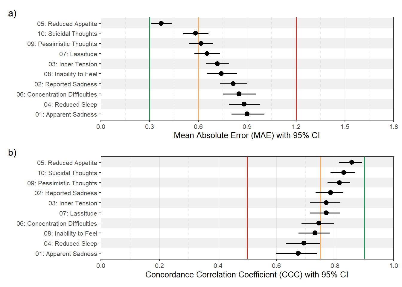

ggsave("best_item.pdf", width = 6.5, height = 6.0, units = "in")

Total Score Results

MAE results table and figure

results[[11]] |> 
  transmute(
    model_name,
    direct = mae_00_direct * 10,
    direct_ci = sprintf("[%.1f, %.1f]", mae_lower_00_direct * 10, mae_upper_00_direct * 10),
    indirect = mae_00_indirect * 10,
    indirect_ci = sprintf("[%.1f, %.1f]", mae_lower_00_indirect * 10, mae_upper_00_indirect * 10),
    diff = diff_mae_obs * 10,
    diff_ci = sprintf("[%.1f, %.1f]", diff_mae_lower * 10, diff_mae_upper * 10),
    p_adj = p.adjust(p_diff_mae, method = "fdr"),
    sig = if_else(p_adj < .05, "*", "")
  ) |> 
  arrange(indirect) |> 
  gt() |> 
  fmt_number(columns = c(direct, indirect, diff), decimals = 1) |> 
  fmt_number(columns = p_adj, decimals = 4) |> 
  cols_align(align = "center", columns = -model_name) |> 
  opt_row_striping() |> 
  tab_options(data_row.padding = px(5))

model_name	direct	direct_ci	indirect	indirect_ci	diff	diff_ci	p_adj	sig
Qwen 3 (22B-235B)	5.2	[4.8, 5.6]	3.5	[3.1, 3.9]	−1.7	[-2.2, -1.2]	0.0000	*
Qwen 2.5 (14B): 1M	5.8	[5.4, 6.3]	3.5	[3.2, 3.8]	−2.3	[-2.8, -1.8]	0.0000	*
DeepSeek R1 Qwen 2.5 (32B)	7.0	[6.5, 7.6]	3.6	[3.2, 3.9]	−3.5	[-4.1, -2.8]	0.0000	*
GPT OSS 120B (5B-117B)	5.7	[5.2, 6.2]	3.6	[3.3, 4.0]	−2.1	[-2.6, -1.6]	0.0000	*
Llama 4 Scout (17B-109B)	5.6	[5.2, 6.0]	3.7	[3.3, 4.0]	−1.9	[-2.3, -1.4]	0.0000	*
Magistral Small 2507 (24B)	7.3	[6.8, 7.8]	3.7	[3.3, 4.1]	−3.6	[-4.4, -2.8]	0.0000	*
DeepSeek R1 Llama 3.3 (70B)	9.2	[8.4, 10.1]	3.7	[3.4, 4.1]	−5.5	[-6.4, -4.6]	0.0000	*
Qwen 2.5 (72B)	5.3	[4.9, 5.8]	3.8	[3.4, 4.1]	−1.6	[-2.0, -1.1]	0.0000	*
Qwen 3 (32B)	10.6	[9.5, 11.8]	3.8	[3.4, 4.2]	−6.8	[-8.1, -5.7]	0.0000	*
GPT OSS 20B (3B-21B)	7.0	[6.4, 7.6]	3.8	[3.4, 4.3]	−3.2	[-3.9, -2.5]	0.0000	*
QwQ (32B)	11.1	[10.2, 12.0]	3.9	[3.6, 4.3]	−7.1	[-8.0, -6.3]	0.0000	*
Qwen 3 (3B-30B)	12.4	[10.8, 14.1]	3.9	[3.5, 4.4]	−8.4	[-10.2, -6.8]	0.0000	*
Qwen 3 (14B)	9.6	[8.9, 10.3]	4.0	[3.6, 4.4]	−5.7	[-6.4, -4.9]	0.0000	*
Llama 4 Maverick (17B-400B)	5.5	[5.1, 5.9]	4.0	[3.6, 4.3]	−1.6	[-2.0, -1.1]	0.0000	*
Qwen 3 (8B)	11.7	[11.0, 12.5]	4.1	[3.8, 4.5]	−7.6	[-8.4, -6.8]	0.0000	*
Qwen 3 Next (80B)	5.3	[4.9, 5.7]	4.1	[3.8, 4.5]	−1.1	[-1.6, -0.7]	0.0000	*
Qwen 3 Next (80B): No Reasoning	8.8	[8.0, 9.6]	4.3	[3.9, 4.7]	−4.5	[-5.3, -3.8]	0.0000	*
Llama 3.3 (70B)	7.1	[6.5, 7.6]	4.6	[4.2, 5.0]	−2.5	[-3.1, -1.9]	0.0000	*
Qwen 2.5 (7B): 1M	5.7	[5.3, 6.2]	4.6	[4.2, 5.0]	−1.2	[-1.6, -0.7]	0.0000	*
Gemma 3 (27B) IT	12.1	[11.3, 12.9]	4.8	[4.3, 5.2]	−7.4	[-8.1, -6.6]	0.0000	*
Qwen 3 (4B)	13.0	[12.1, 13.8]	5.3	[4.9, 5.8]	−7.6	[-8.5, -6.8]	0.0000	*
Qwen 3 (1.7B)	10.6	[9.8, 11.3]	7.1	[6.6, 7.8]	−3.4	[-4.4, -2.4]	0.0000	*
Llama 3.1 (8B)	12.7	[11.8, 13.6]	8.0	[7.4, 8.7]	−4.6	[-5.4, -3.8]	0.0000	*
Qwen 3 (0.6B)	15.8	[14.7, 16.9]	9.3	[8.6, 10.0]	−6.5	[-7.4, -5.6]	0.0000	*
DeepSeek R1 Llama 3.1 (8B)	11.4	[10.6, 12.2]	11.8	[11.1, 12.6]	0.4	[-0.4, 1.3]	0.3045

bench1 <- 12
bench2 <- 06
bench3 <- 03

total_plot_data <- 
  results[[11]] |> 
  transmute(
    model_name,
    mae = mae_00_indirect * 10,
    mae_lower = mae_lower_00_indirect * 10,
    mae_upper = mae_upper_00_indirect * 10
  )

stripe_df <- 
  total_plot_data |> 
  mutate(
    model = fct_reorder(model_name, .x = mae, .desc = TRUE),
    y_id  = as.numeric(model)
  ) |>
  filter(y_id %% 2 == 0) |>
  transmute(
    ymin = y_id - 0.5,
    ymax = y_id + 0.5,
    xmin = -Inf,
    xmax =  Inf
  )

p1 <- 
  total_plot_data |> 
  mutate(
    model = fct_reorder(model_name, .x = mae, .desc = TRUE),
  ) |> 
  ggplot( 
    aes(
      x    = mae, 
      xmin = mae_lower, 
      xmax = mae_upper, 
      y    = model
    )
  ) +
  geom_rect(
    data        = stripe_df,
    aes(xmin = xmin, xmax = xmax, ymin = ymin, ymax = ymax),
    inherit.aes = FALSE,
    fill        = "grey80",
    alpha       = 0.3
  ) +
  geom_vline(xintercept = bench1, color = "#D73027", linewidth = 2/3) +
  geom_vline(xintercept = bench2, color = "#FDAE61", linewidth = 2/3) +
  geom_vline(xintercept = bench3, color = "#1A9850", linewidth = 2/3) +
  geom_pointrange(linewidth = 2/3) +
  scale_x_continuous(
    limits = c(0, 15),
    expand = c(0, 0),
    breaks = seq(0, 15, 3)
  ) +
  labs(x = "Mean Absolute Error (MAE) with 95% CI", y = NULL) +
  theme_bw(base_size = 10) +
  theme(
    panel.grid.major.y = element_blank(),
    panel.grid.minor.y = element_blank(),
    panel.grid.major.x = element_line(linewidth = 1/2, linetype = "solid"),
    panel.grid.minor.x = element_line(linewidth = 1/2, linetype = "dashed")
  )
p1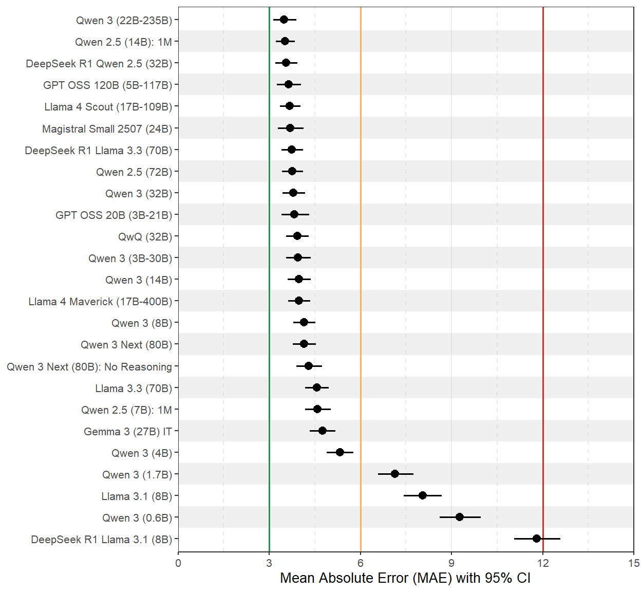

ggsave("mae_indirect.pdf", width = 6.5, height = 6.0, units = "in")

CCC results table and figure

results[[11]] |> 
  transmute(
    model_name,
    direct = ccc_00_direct,
    direct_ci = sprintf("[%.2f, %.2f]", ccc_lower_00_direct, ccc_upper_00_direct),
    indirect = ccc_00_indirect,
    indirect_ci = sprintf("[%.2f, %.2f]", ccc_lower_00_indirect, ccc_upper_00_indirect),
    diff = diff_ccc_obs,
    diff_ci = sprintf("[%.2f, %.2f]", diff_ccc_lower, diff_ccc_upper),
    p_adj = p.adjust(p_diff_ccc, method = "fdr"),
    sig = if_else(p_adj < .05, "*", "")
  ) |> 
  arrange(desc(indirect)) |> 
  gt() |> 
  fmt_number(columns = c(direct, indirect, diff), decimals = 2) |> 
  fmt_number(columns = p_adj, decimals = 3) |> 
  cols_align(align = "center", columns = -model_name) |> 
  opt_row_striping() |> 
  tab_options(data_row.padding = px(5))

model_name	direct	direct_ci	indirect	indirect_ci	diff	diff_ci	p_adj	sig
Qwen 2.5 (14B): 1M	0.80	[0.77, 0.83]	0.91	[0.89, 0.93]	0.11	[0.08, 0.15]	0.000	*
Llama 4 Scout (17B-109B)	0.80	[0.77, 0.83]	0.90	[0.88, 0.92]	0.11	[0.07, 0.14]	0.000	*
Qwen 3 (22B-235B)	0.86	[0.84, 0.88]	0.90	[0.87, 0.92]	0.04	[0.01, 0.07]	0.004	*
DeepSeek R1 Qwen 2.5 (32B)	0.68	[0.62, 0.73]	0.90	[0.87, 0.92]	0.22	[0.16, 0.29]	0.000	*
DeepSeek R1 Llama 3.3 (70B)	0.66	[0.59, 0.71]	0.90	[0.87, 0.92]	0.24	[0.18, 0.31]	0.000	*
Qwen 2.5 (72B)	0.84	[0.80, 0.86]	0.90	[0.87, 0.92]	0.06	[0.04, 0.09]	0.000	*
Magistral Small 2507 (24B)	0.73	[0.69, 0.76]	0.89	[0.86, 0.92]	0.17	[0.12, 0.21]	0.000	*
GPT OSS 120B (5B-117B)	0.81	[0.77, 0.84]	0.89	[0.86, 0.92]	0.08	[0.05, 0.11]	0.000	*
Llama 4 Maverick (17B-400B)	0.82	[0.79, 0.85]	0.89	[0.86, 0.91]	0.07	[0.04, 0.10]	0.000	*
Qwen 3 (32B)	0.46	[0.37, 0.54]	0.89	[0.86, 0.91]	0.43	[0.34, 0.52]	0.000	*
Qwen 3 (14B)	0.62	[0.56, 0.67]	0.89	[0.86, 0.91]	0.27	[0.22, 0.32]	0.000	*
QwQ (32B)	0.53	[0.45, 0.60]	0.89	[0.86, 0.91]	0.35	[0.29, 0.43]	0.000	*
Qwen 3 Next (80B)	0.86	[0.83, 0.88]	0.89	[0.86, 0.91]	0.03	[0.01, 0.05]	0.013	*
Qwen 3 (3B-30B)	0.30	[0.16, 0.43]	0.89	[0.85, 0.91]	0.59	[0.46, 0.73]	0.000	*
Qwen 3 Next (80B): No Reasoning	0.70	[0.66, 0.74]	0.88	[0.85, 0.91]	0.18	[0.14, 0.22]	0.000	*
Qwen 3 (8B)	0.54	[0.49, 0.59]	0.88	[0.85, 0.90]	0.34	[0.29, 0.39]	0.000	*
GPT OSS 20B (3B-21B)	0.78	[0.74, 0.81]	0.88	[0.84, 0.91]	0.10	[0.06, 0.14]	0.000	*
Llama 3.3 (70B)	0.77	[0.73, 0.81]	0.88	[0.85, 0.90]	0.10	[0.07, 0.14]	0.000	*
Qwen 2.5 (7B): 1M	0.81	[0.78, 0.84]	0.86	[0.83, 0.89]	0.05	[0.03, 0.08]	0.000	*
Gemma 3 (27B) IT	0.57	[0.52, 0.61]	0.86	[0.83, 0.89]	0.29	[0.26, 0.33]	0.000	*
Qwen 3 (4B)	0.45	[0.40, 0.51]	0.83	[0.79, 0.86]	0.37	[0.33, 0.42]	0.000	*
Llama 3.1 (8B)	0.53	[0.49, 0.58]	0.73	[0.69, 0.77]	0.20	[0.17, 0.23]	0.000	*
Qwen 3 (1.7B)	0.25	[0.16, 0.34]	0.70	[0.64, 0.74]	0.44	[0.35, 0.54]	0.000	*
DeepSeek R1 Llama 3.1 (8B)	0.49	[0.44, 0.55]	0.50	[0.44, 0.55]	0.00	[-0.04, 0.05]	0.848
Qwen 3 (0.6B)	−0.14	[-0.21, -0.07]	0.46	[0.40, 0.51]	0.60	[0.50, 0.69]	0.000	*

# Plot of best model
bench1 <- 0.50
bench2 <- 0.75
bench3 <- 0.90

total_plot_data <- 
  results[[11]] |> 
  transmute(
    model_name,
    ccc = ccc_00_indirect,
    ccc_lower = ccc_lower_00_indirect,
    ccc_upper = ccc_upper_00_indirect
  )

stripe_df <- 
  total_plot_data |> 
  mutate(
    model = fct_reorder(model_name, .x = ccc, .desc = FALSE),
    y_id  = as.numeric(model)
  ) |>
  filter(y_id %% 2 == 0) |>
  transmute(
    ymin = y_id - 0.5,
    ymax = y_id + 0.5,
    xmin = -Inf,
    xmax =  Inf
  )

p1 <- 
  total_plot_data |> 
  mutate(
    model = fct_reorder(model_name, .x = ccc, .desc = FALSE),
  ) |> 
  ggplot( 
    aes(
      x    = ccc, 
      xmin = ccc_lower, 
      xmax = ccc_upper, 
      y    = model
    )
  ) +
  geom_rect(
    data = stripe_df,
    aes(xmin = xmin, xmax = xmax, ymin = ymin, ymax = ymax),
    inherit.aes = FALSE,
    fill = "grey80",
    alpha = 0.3
  ) +
  geom_vline(xintercept = bench1, color = "#D73027", linewidth = 2/3) +
  geom_vline(xintercept = bench2, color = "#FDAE61", linewidth = 2/3) +
  geom_vline(xintercept = bench3, color = "#1A9850", linewidth = 2/3) +
  geom_pointrange(linewidth = 2/3) +
  scale_x_continuous(
    limits = c(0, 1),
    expand = c(0, 0),
    breaks = seq(0, 1, 0.2)
  ) +
  labs(x = "Concordance Correlation Coefficient (CCC) with 95% CI", y = NULL) +
  theme_bw(base_size = 10) +
  theme(
    panel.grid.major.y = element_blank(),
    panel.grid.minor.y = element_blank(),
    panel.grid.major.x = element_line(linewidth = 1/2, linetype = "solid"),
    panel.grid.minor.x = element_line(linewidth = 1/2, linetype = "dashed")
  )
p1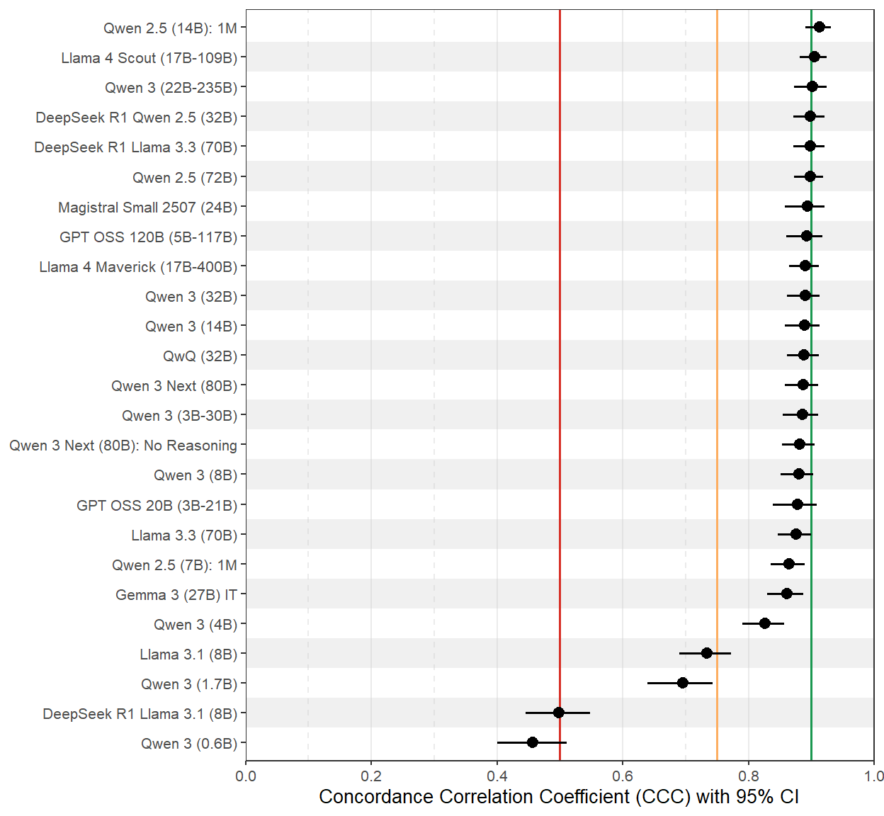

ggsave("ccc_indirect.pdf", width = 6.5, height = 6.0, units = "in")

Directional Error

best_model_data <- 
  fewshot_all |>
  filter(model_name == "Qwen 3 (22B-235B)") |>
  mutate(
    # Multiply by 10 to convert back to the 0-60 total score scale
    label = label00 * 10,
    pred = indirect00 * 10
  )
directional_summary <- 
  best_model_data |>
  mutate(
    severity_bin = case_when(
      label <= 6 ~ "Normal (0-6)",
      label >= 7 & label <= 19 ~ "Mild (7-19)",
      label >= 20 & label <= 34 ~ "Moderate (20-34)",
      label >= 35 ~ "Severe (35-60)",
      .default = NA_character_
    ),
    severity_bin = fct_relevel(
      severity_bin, 
      "Normal (0-6)", "Mild (7-19)", "Moderate (20-34)", "Severe (35-60)"
    ),
    error = pred - label,
    abs_error = abs(error)
  ) |>
  filter(!is.na(severity_bin)) |>
  summarize(
    .by = severity_bin,
    mean_error = mean(error, na.rm = TRUE),
    mae = mean(abs_error, na.rm = TRUE),
    n = n()
  ) |> 
  arrange(severity_bin)

# Create the styled gt table
directional_summary |>
  gt() |>
  tab_header(
    title = "Directional Error Analysis by Clinical Severity",
    subtitle = "Analysis of Prediction Bias and Accuracy for Qwen 3 (22B-235B)"
  ) |>
  cols_label(
    severity_bin = "Severity Range",
    mean_error = "Mean Error (Bias)",
    mae = "MAE",
    n = "Sample Size (N)"
  ) |>
  fmt_number(
    columns = c(mean_error, mae),
    decimals = 2
  ) |>
  # Apply a color scale to Mean Error to highlight over/underestimation
  data_color(
    columns = mean_error,
    palette = c("#2166ac", "white", "#b2182b"), # Blue (under) to Red (over)
    domain = c(-6, 6) # Adjust this range based on your typical error spread
  ) |>
  cols_align(
    align = "center",
    columns = -severity_bin
  ) |>
  tab_source_note(
    source_note = "Note: Positive Mean Error indicates overestimation; negative indicates underestimation."
  ) |>
  opt_row_striping() |>
  tab_options(
    heading.title.font.size = px(20),
    column_labels.font.weight = "bold",
    data_row.padding = px(8)
  )

Directional Error Analysis by Clinical Severity
Analysis of Prediction Bias and Accuracy for Qwen 3 (22B-235B)
Severity Range	Mean Error (Bias)	MAE	Sample Size (N)
Normal (0-6)	1.61	2.12	77
Mild (7-19)	0.08	3.17	195
Moderate (20-34)	−1.88	3.61	192
Severe (35-60)	−5.44	5.80	74
Note: Positive Mean Error indicates overestimation; negative indicates underestimation.