Code
library(tidyverse)
library(easystats)
library(brms)
library(ordbetareg)
library(flextable)
library(patchwork)library(tidyverse)
library(easystats)
library(brms)
library(ordbetareg)
library(flextable)
library(patchwork)# Deidentified features (one row per participant and task); see ../data/README.md
df_verbal <-
# base R's parser restores every stored value exactly (readr's can differ in the last digit)
read.csv(file.path("..", "data", "verbal.csv")) |>
as_tibble() |>
mutate(
participant = factor(participant),
source = factor(source, levels = c("clinic", "prolific")),
ptsd = factor(ptsd, levels = c(0, 1)),
demo_sex = factor(demo_sex, levels = c("Male", "Female")),
demo_nonwhite = factor(demo_nonwhite, levels = c(FALSE, TRUE)),
task = factor(task, levels = c("Account", "Impact")),
# LIWC percentages to proportions
across(c(i, we, emo_neg, emo_pos, allnone, cogproc, Perception), \(x) x / 100),
sentiment_num = sentiment,
sentiment = factor(
sentiment_num,
levels = 1:6,
ordered = TRUE
)
) |>
arrange(participant, task)
# Effect-code every two-level factor (first level = -0.5, second = +0.5) so each main effect is averaged
# over the other factors (e.g., group = PTSD - Control averaged across tasks); interactions and predictions are unchanged
for (v in c("task", "ptsd", "demo_sex", "demo_nonwhite")) contrasts(df_verbal[[v]]) <- c(-0.5, 0.5)
dir.create("fits", showWarnings = FALSE)
df_verbal |>
select(WC:Perception, sentiment_num) |>
pivot_longer(cols = everything()) |>
ggplot(aes(x = value)) +
facet_wrap(~name, scales = "free") +
geom_histogram(bins = 30)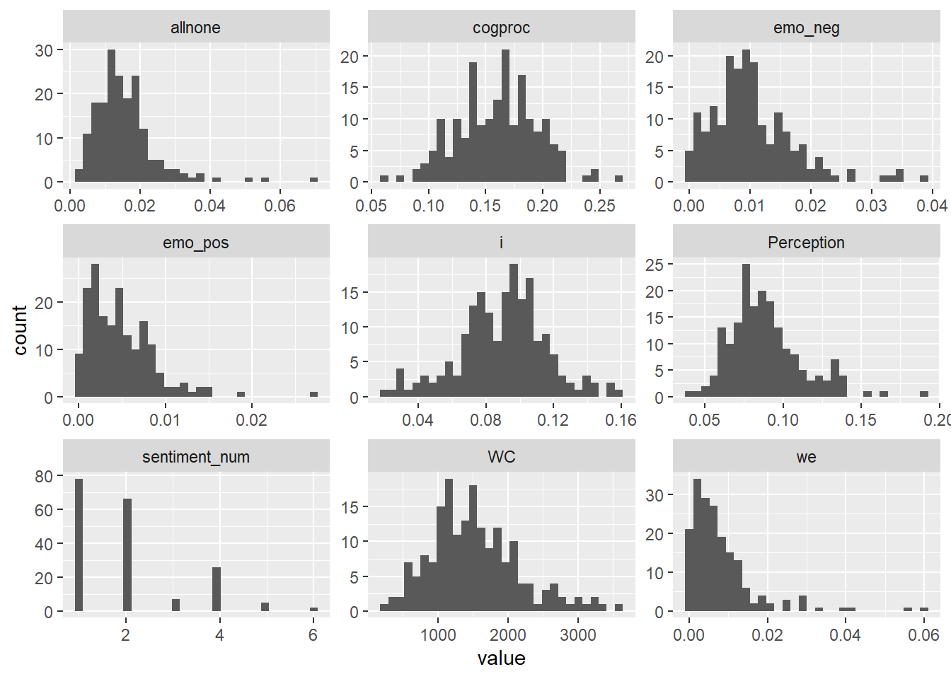
# models with divergent transitions at adapt_delta = 0.95
high_adapt <- c("we")

ob_features <- c(
  "i", "we",
  "emo_neg", "emo_pos",
  "allnone", "cogproc",
  "Perception"
)

ob_models <-
  ob_features |>
  set_names() |>
  map(
    \(feature) {
      model_formula <- as.formula(
        paste(feature, "~ task * ptsd + demo_age + demo_sex + demo_nonwhite + (1 | participant)")
      )
      ordbetareg(
        formula = model_formula,
        data = df_verbal,
        coef_prior_mean = 0,
        coef_prior_SD = 1,
        seed = 2026,
        chains = 4,
        cores = 4,
        iter = 4000,
        warmup = 2000,
        refresh = 0,
        file = file.path("fits", feature),
        control = list(adapt_delta = if (feature %in% high_adapt) 0.99 else 0.95, max_treedepth = 12),
        backend = "cmdstanr"
      )
    }
  )

iwalk(
  ob_models,
  \(model, name) {
    thisr2 <- r2(model)
    cat(
      "\n\n#### ",
      name,
      sprintf("(R2C = %0.2f, R2M = %0.2f)", thisr2$R2_Bayes, thisr2$R2_Bayes_marginal),
      "\n\n"
    )
    table_md <- print_md(model_parameters(model))
    cat(table_md, sep = "\n")
  }
)| Parameter | Median | 95% CI | pd | Rhat | ESS (tail) |
|---|---|---|---|---|---|
| (Intercept) | -2.26 | (-2.43, -2.09) | 100% | 1.000 | 7015 |
| task1 | 0.08 | (1.38e-03, 0.17) | 97.69% | 1.000 | 5826 |
| ptsd1 | 0.13 | (0.01, 0.25) | 98.40% | 1.000 | 6137 |
| demo_age | -1.80e-03 | (-5.71e-03, 2.16e-03) | 81.80% | 1.000 | 6911 |
| demo_sex1 | 0.25 | (0.13, 0.37) | 100% | 1.001 | 6119 |
| demo_nonwhite1 | 0.12 | (-0.01, 0.26) | 96.53% | 1.000 | 5823 |
| task1:ptsd1 | 0.07 | (-0.10, 0.23) | 79.54% | 1.001 | 5513 |
| Parameter | Median | 95% CI | pd | Rhat | ESS (tail) |
|---|---|---|---|---|---|
| (Intercept) | -5.15 | (-5.59, -4.71) | 100% | 1.000 | 4997 |
| task1 | -0.54 | (-0.75, -0.34) | 100% | 1.000 | 5923 |
| ptsd1 | -0.03 | (-0.32, 0.26) | 58.76% | 1.001 | 4961 |
| demo_age | 8.38e-03 | (-1.19e-03, 0.02) | 95.73% | 1.000 | 6279 |
| demo_sex1 | -0.31 | (-0.60, -0.04) | 98.61% | 1.000 | 4892 |
| demo_nonwhite1 | -0.11 | (-0.49, 0.25) | 71.75% | 1.001 | 5733 |
| task1:ptsd1 | -0.19 | (-0.58, 0.22) | 81.97% | 1.000 | 4899 |
| Parameter | Median | 95% CI | pd | Rhat | ESS (tail) |
|---|---|---|---|---|---|
| (Intercept) | -4.39 | (-4.68, -4.11) | 100% | 1.000 | 6458 |
| task1 | -0.47 | (-0.64, -0.30) | 100% | 1.001 | 5830 |
| ptsd1 | 0.25 | (0.05, 0.47) | 99.10% | 1.001 | 6515 |
| demo_age | -8.04e-03 | (-0.01, -1.73e-03) | 99.38% | 1.001 | 6777 |
| demo_sex1 | 0.21 | (3.10e-03, 0.43) | 97.71% | 1.000 | 6665 |
| demo_nonwhite1 | -0.34 | (-0.61, -0.10) | 99.69% | 1.000 | 6155 |
| task1:ptsd1 | 0.51 | (0.17, 0.85) | 99.83% | 1.001 | 6521 |
| Parameter | Median | 95% CI | pd | Rhat | ESS (tail) |
|---|---|---|---|---|---|
| (Intercept) | -5.17 | (-5.54, -4.81) | 100% | 1.000 | 6322 |
| task1 | 0.26 | (0.05, 0.46) | 99.24% | 1.001 | 6389 |
| ptsd1 | 0.11 | (-0.13, 0.36) | 80.95% | 1.000 | 5958 |
| demo_age | -7.45e-04 | (-8.84e-03, 7.23e-03) | 57.01% | 1.000 | 6093 |
| demo_sex1 | 0.03 | (-0.22, 0.29) | 59.19% | 1.000 | 6200 |
| demo_nonwhite1 | 0.05 | (-0.25, 0.32) | 62.26% | 1.001 | 5584 |
| task1:ptsd1 | 0.32 | (-0.10, 0.71) | 93.38% | 1.001 | 5472 |
| Parameter | Median | 95% CI | pd | Rhat | ESS (tail) |
|---|---|---|---|---|---|
| (Intercept) | -4.44 | (-4.72, -4.16) | 100% | 1.000 | 6702 |
| task1 | 0.21 | (0.06, 0.37) | 99.72% | 1.000 | 5525 |
| ptsd1 | 0.19 | (5.66e-03, 0.38) | 97.82% | 1.000 | 6297 |
| demo_age | 8.22e-03 | (1.86e-03, 0.01) | 99.45% | 1.000 | 6674 |
| demo_sex1 | -0.03 | (-0.21, 0.16) | 61.82% | 1.001 | 6268 |
| demo_nonwhite1 | 0.12 | (-0.10, 0.33) | 86.71% | 1.000 | 6551 |
| task1:ptsd1 | 0.31 | (1.75e-03, 0.60) | 97.55% | 1.002 | 5639 |
| Parameter | Median | 95% CI | pd | Rhat | ESS (tail) |
|---|---|---|---|---|---|
| (Intercept) | -1.55 | (-1.67, -1.43) | 100% | 1.000 | 6680 |
| task1 | 0.32 | (0.26, 0.39) | 100% | 1.001 | 5461 |
| ptsd1 | -0.09 | (-0.17, 2.87e-03) | 97.11% | 1.001 | 6220 |
| demo_age | -3.08e-03 | (-5.92e-03, -2.64e-04) | 98.41% | 1.000 | 6232 |
| demo_sex1 | 0.03 | (-0.06, 0.11) | 72.32% | 1.000 | 5913 |
| demo_nonwhite1 | -0.03 | (-0.14, 0.08) | 71.30% | 1.001 | 5983 |
| task1:ptsd1 | 0.02 | (-0.10, 0.14) | 61.81% | 1.000 | 5976 |
| Parameter | Median | 95% CI | pd | Rhat | ESS (tail) |
|---|---|---|---|---|---|
| (Intercept) | -2.55 | (-2.69, -2.41) | 100% | 1.001 | 6754 |
| task1 | -0.19 | (-0.27, -0.12) | 100% | 1.001 | 5827 |
| ptsd1 | -0.05 | (-0.15, 0.05) | 84.34% | 1.001 | 6626 |
| demo_age | 4.81e-03 | (1.56e-03, 8.04e-03) | 99.84% | 1.000 | 6686 |
| demo_sex1 | 0.01 | (-0.09, 0.12) | 60.62% | 1.001 | 6282 |
| demo_nonwhite1 | -0.04 | (-0.16, 0.08) | 72.97% | 1.000 | 6562 |
| task1:ptsd1 | -0.03 | (-0.17, 0.12) | 63.99% | 1.001 | 5763 |
wc_model <-
  brm(
    formula = WC ~ task * ptsd + demo_age + demo_sex + demo_nonwhite + (1 | participant),
    data = df_verbal,
    family = negbinomial(),
    prior = set_prior("normal(0, 1)", class = "b"),
    seed = 2026,
    chains = 4,
    cores = 4,
    iter = 4000,
    warmup = 2000,
    refresh = 0,
    file = file.path("fits", "WC"),
    control = list(adapt_delta = 0.95, max_treedepth = 12),
    backend = "cmdstanr"
  )

r2(wc_model)
# Bayesian R2 with Compatibility Interval
Conditional R2: 0.607 (95% CI [0.500, 0.697])
Marginal R2: 0.167 (95% CI [0.064, 0.274])model_parameters(wc_model) |> print_md()| Parameter | Median | 95% CI | pd | Rhat | ESS (tail) |
|---|---|---|---|---|---|
| (Intercept) | 7.43 | (7.17, 7.68) | 100% | 1.001 | 4480 |
| task1 | 0.04 | (-0.04, 0.12) | 82.16% | 1.000 | 6119 |
| ptsd1 | 0.21 | (0.01, 0.40) | 98.12% | 1.002 | 3995 |
| demo_age | -3.01e-03 | (-8.72e-03, 2.84e-03) | 83.81% | 1.001 | 4810 |
| demo_sex1 | 0.09 | (-0.10, 0.28) | 82.19% | 1.001 | 3896 |
| demo_nonwhite1 | 0.13 | (-0.09, 0.34) | 87.59% | 1.002 | 4871 |
| task1:ptsd1 | 0.11 | (-0.06, 0.27) | 89.35% | 1.000 | 5765 |
sentiment_model <-
  brm(
    formula = sentiment ~ task * ptsd + demo_age + demo_sex + demo_nonwhite + (1 | participant),
    data = df_verbal,
    family = cumulative(link = "logit", link_disc = "log"),
    # wider prior: task and group effects are ~2-2.5 on the logit scale, so normal(0, 1) shrank them
    prior = set_prior("normal(0, 2.5)", class = "b"),
    seed = 2026,
    chains = 4,
    cores = 4,
    iter = 4000,
    warmup = 2000,
    refresh = 0,
    file = file.path("fits", "sentiment"),
    file_refit = "on_change",
    control = list(adapt_delta = 0.95, max_treedepth = 12),
    backend = "cmdstanr"
  )

r2_latent <- function(model, link_var = pi^2 / 3) {
  eta_fixed <- posterior_linpred(model, re_formula = NA)
  var_fixed <- apply(eta_fixed, 1, var)
  var_re <- as_draws_matrix(model, variable = "sd_participant__Intercept")[, 1]^2
  denom <- var_fixed + var_re + link_var
  r2c <- (var_fixed + var_re) / denom
  r2m <- var_fixed / denom
  tibble(
    Statistic = c("R2 (conditional)", "R2 (marginal)"),
    Median  = c(median(r2c), median(r2m)),
    CI_low  = c(quantile(r2c, 0.025), quantile(r2m, 0.025)),
    CI_high = c(quantile(r2c, 0.975), quantile(r2m, 0.975))
  )
}

r2_latent(sentiment_model)
# A tibble: 2 × 4
Statistic Median CI_low CI_high
<chr> <dbl> <dbl> <dbl>
1 R2 (conditional) 0.696 0.540 0.805
2 R2 (marginal) 0.548 0.435 0.641model_parameters(sentiment_model) |> print_md()| Parameter | Median | 95% CI | pd | Rhat | ESS (tail) |
|---|---|---|---|---|---|
| Intercept(1) | 0.43 | (-0.92, 1.86) | 72.79% | 1.000 | 5427 |
| Intercept(2) | 3.59 | (2.16, 5.40) | 100% | 1.000 | 4651 |
| Intercept(3) | 4.10 | (2.62, 5.98) | 100% | 1.000 | 4477 |
| Intercept(4) | 6.90 | (5.02, 9.42) | 100% | 1.001 | 4220 |
| Intercept(5) | 8.69 | (6.38, 11.79) | 100% | 1.001 | 4896 |
| task1 | 2.92 | (2.12, 3.93) | 100% | 1.000 | 4328 |
| ptsd1 | -2.61 | (-3.85, -1.58) | 100% | 1.000 | 3694 |
| demo_age | 0.03 | (2.47e-03, 0.07) | 98.15% | 1.000 | 4431 |
| demo_sex1 | -1.14 | (-2.19, -0.18) | 99.08% | 1.000 | 5751 |
| demo_nonwhite1 | -0.19 | (-1.43, 0.98) | 62.90% | 1.001 | 6281 |
| task1:ptsd1 | -0.44 | (-1.81, 0.94) | 74.05% | 1.001 | 6357 |
wc_list <- list("Word Count" = wc_model)
sentiment_list <- list("Sentiment" = sentiment_model)
all_models <- c(ob_models, wc_list, sentiment_list)

extract_model_stats <- function(model, model_name) {

  describe_posterior(model, effects = "fixed", component = "conditional", test = "pd") |>
    as_tibble() |>
    filter(str_detect(Parameter, "task|ptsd")) |>
    mutate(
      stars = case_when(
        pd >= 0.995 ~ "***",
        pd >= 0.985 ~ "**",
        pd >= 0.975 ~ "*",
        TRUE        ~ ""
      ),
      formatted_stat = sprintf("%.2f [%.2f, %.2f]%s", Median, CI_low, CI_high, stars),

      Term = case_when(
        str_detect(Parameter, ":") ~ "Interaction",
        str_detect(Parameter, "task") ~ "Main_Task",
        str_detect(Parameter, "ptsd") ~ "Main_PTSD",
        TRUE ~ Parameter
      )
    ) |>
    select(Term, formatted_stat) |>
    pivot_wider(names_from = Term, values_from = formatted_stat) |>
    mutate(Feature = model_name, .before = 1)
}

table_data <- imap(all_models, \(model, name) extract_model_stats(model, name)) |>
  list_rbind()

final_table <-
  flextable(table_data) |>
  set_header_labels(
    Feature = "Feature",
    Main_Task = "Main Effect: Task",
    Main_PTSD = "Main Effect: PTSD",
    Interaction = "Task × PTSD Effect"
  ) |>
  autofit() |>
  add_footer_lines("Note: Estimates are median posterior values on the link scale (identity, log, or logit). Models control for age, sex, and race. Brackets indicate 95% Credible Intervals. * pd > 97.5%, ** pd > 98.5%, *** pd > 99.5%. ")

final_table
Feature | Main Effect: Task | Main Effect: PTSD | Task × PTSD Effect |
|---|---|---|---|
i | 0.08 [0.00, 0.17]* | 0.13 [0.01, 0.25]* | 0.07 [-0.10, 0.23] |
we | -0.54 [-0.75, -0.34]*** | -0.03 [-0.32, 0.26] | -0.19 [-0.58, 0.22] |
emo_neg | -0.47 [-0.64, -0.30]*** | 0.25 [0.05, 0.47]** | 0.51 [0.17, 0.85]*** |
emo_pos | 0.26 [0.05, 0.46]** | 0.11 [-0.13, 0.36] | 0.32 [-0.10, 0.71] |
allnone | 0.21 [0.06, 0.37]*** | 0.19 [0.01, 0.38]* | 0.31 [0.00, 0.60]* |
cogproc | 0.32 [0.26, 0.39]*** | -0.09 [-0.17, 0.00] | 0.02 [-0.10, 0.14] |
Perception | -0.19 [-0.27, -0.12]*** | -0.05 [-0.15, 0.05] | -0.03 [-0.17, 0.12] |
Word Count | 0.04 [-0.04, 0.12] | 0.21 [0.01, 0.40]* | 0.11 [-0.06, 0.27] |
Sentiment | 2.92 [2.12, 3.93]*** | -2.61 [-3.85, -1.58]*** | -0.44 [-1.81, 0.94] |
Note: Estimates are median posterior values on the link scale (identity, log, or logit). Models control for age, sex, and race. Brackets indicate 95% Credible Intervals. * pd > 97.5%, ** pd > 98.5%, *** pd > 99.5%. | |||
# Simple group effects (PTSD - Control) within each task on the response scale,
# averaged over sex and race (equal weights, matching the effect coding) at the
# mean age, with random intercepts at zero
extract_group_deltas <- function(model, model_name) {
  if (model_name == "Sentiment") {
    # estimate_contrasts() works per rating category for the ordinal model, so
    # compare expected ratings, computed per posterior draw
    probs <- estimate_means(model, by = c("task", "ptsd"), re_formula = NA, keep_iterations = TRUE) |>
      as.data.frame()
    iters <- grep("^iter_", names(probs), value = TRUE)
    out <- probs |>
      mutate(Response = as.numeric(as.character(Response))) |>
      summarize(.by = c(task, ptsd), across(all_of(iters), \(p) sum(Response * p))) |>
      pivot_longer(all_of(iters), names_to = "draw") |>
      pivot_wider(names_from = ptsd, values_from = value) |>
      mutate(diff = `1` - `0`) |>
      summarize(
        .by = task,
        Estimate = median(diff),
        CI_Low = quantile(diff, 0.025),
        CI_High = quantile(diff, 0.975),
        pd = max(mean(diff > 0), mean(diff < 0))
      ) |>
      transmute(Feature = model_name, Task = as.character(task), Estimate, CI_Low, CI_High, pd)
    return(out)
  }
  ec <- estimate_contrasts(model, contrast = "ptsd", by = "task", re_formula = NA) |>
    as.data.frame()
  stopifnot(all(ec$Level1 == "1" & ec$Level2 == "0"))  # PTSD minus Control
  ec |>
    transmute(
      Feature = model_name,
      Task = as.character(task),
      Estimate = Median,
      CI_Low = CI_low,
      CI_High = CI_high,
      pd
    )
}

group_delta_results <- imap(all_models, \(model, name) {
  extract_group_deltas(model, name)
}) |> list_rbind()

group_delta_table <- group_delta_results |>
  mutate(Feature = gsub("_", " ", Feature)) |>
  flextable() |>
  colformat_double(
    j = c("Estimate", "CI_Low", "CI_High"),
    digits = 3
  ) |>
  colformat_double(
    j = "pd",
    digits = 3
  ) |>
  set_header_labels(
    Feature = "Feature",
    Task = "Task",
    Estimate = "PTSD Δ", # PTSD minus Control
    CI_Low = "Lower 95% CI",
    CI_High = "Upper 95% CI",
    pd = "pd"
  ) |>
  autofit() |>
  italic(j = "pd", part = "header") |>
  bold(i = ~ pd > 0.975, j = c("Estimate", "pd")) |>
  add_footer_lines("Note: PTSD Δ is the estimated difference (PTSD - Control) on the response scale, averaged over sex and race at the mean age. pd = Probability of Direction. Bold rows indicate pd > 0.975.")

group_delta_table
Feature | Task | PTSD Δ | Lower 95% CI | Upper 95% CI | pd |
|---|---|---|---|---|---|
i | Account | 0.008 | -0.004 | 0.021 | 0.905 |
i | Impact | 0.015 | 0.002 | 0.028 | 0.988 |
we | Account | 0.001 | -0.004 | 0.006 | 0.641 |
we | Impact | -0.001 | -0.004 | 0.002 | 0.742 |
emo neg | Account | -0.000 | -0.004 | 0.004 | 0.509 |
emo neg | Impact | 0.004 | 0.002 | 0.009 | 1.000 |
emo pos | Account | -0.000 | -0.003 | 0.002 | 0.609 |
emo pos | Impact | 0.002 | -0.000 | 0.007 | 0.957 |
allnone | Account | 0.001 | -0.004 | 0.005 | 0.616 |
allnone | Impact | 0.007 | 0.002 | 0.015 | 0.998 |
cogproc | Account | -0.011 | -0.025 | 0.002 | 0.952 |
cogproc | Impact | -0.012 | -0.027 | 0.004 | 0.922 |
Perception | Account | -0.003 | -0.014 | 0.008 | 0.727 |
Perception | Impact | -0.005 | -0.015 | 0.005 | 0.839 |
Word Count | Account | 231.177 | -79.740 | 546.548 | 0.934 |
Word Count | Impact | 400.549 | 76.342 | 736.759 | 0.992 |
Sentiment | Account | -0.605 | -0.926 | -0.297 | 1.000 |
Sentiment | Impact | -1.323 | -1.832 | -0.804 | 1.000 |
Note: PTSD Δ is the estimated difference (PTSD - Control) on the response scale, averaged over sex and race at the mean age. pd = Probability of Direction. Bold rows indicate pd > 0.975. | |||||
plot_titles <- c(
  "LIWC: First-Person Singular",
  "LIWC: First-Person Plural",
  "LIWC: Negative Emotion",
  "LIWC: Positive Emotion",
  "LIWC: All-or-None",
  "LIWC: Cognitive Processes",
  "LIWC: Perceptual Processes",
  "Word Count",
  "Sentiment"
)

# Plot the simple group effects from the table above: PTSD minus Control within
# each task, with 95% credible intervals; filled points have pd > 97.5%
make_model_plot <- function(name, title) {
  d <- group_delta_results |>
    filter(Feature == name) |>
    mutate(
      Task = factor(Task, levels = c("Account", "Impact")),
      credible = factor(pd > 0.975, levels = c(FALSE, TRUE), labels = c("No", "Yes"))
    )
  ggplot(d, aes(x = Task, y = Estimate, group = 1)) +
    geom_hline(yintercept = 0, linetype = "dashed", color = "grey50") +
    geom_line(color = "grey40") +
    geom_pointrange(
      aes(ymin = CI_Low, ymax = CI_High, fill = credible),
      shape = 21, size = 0.4, color = "grey20", show.legend = TRUE
    ) +
    scale_fill_manual(values = c(No = "white", Yes = "black"), limits = c("No", "Yes"), drop = FALSE) +
    # typographic minus signs on the y-axis (Cairo otherwise draws a hyphen)
    scale_y_continuous(labels = \(x) sub("^-", "\u2212", format(x, trim = TRUE))) +
    labs(title = title, x = NULL, y = "PTSD − Control Difference (95% CI)", fill = "pd > 97.5%") +
    theme_minimal(base_size = 8) +
    theme(
      plot.title = element_text(size = 9, face = "bold"),
      axis.text.x = element_text(size = 8),
      panel.grid.minor = element_blank(),
      panel.grid.major.x = element_blank()
    )
}

plot_list <- map2(names(all_models), plot_titles, make_model_plot)

combined_plot <- wrap_plots(plot_list, ncol = 3) +
  plot_layout(guides = "collect", axis_titles = "collect") &
  theme(legend.position = "bottom")

combined_plot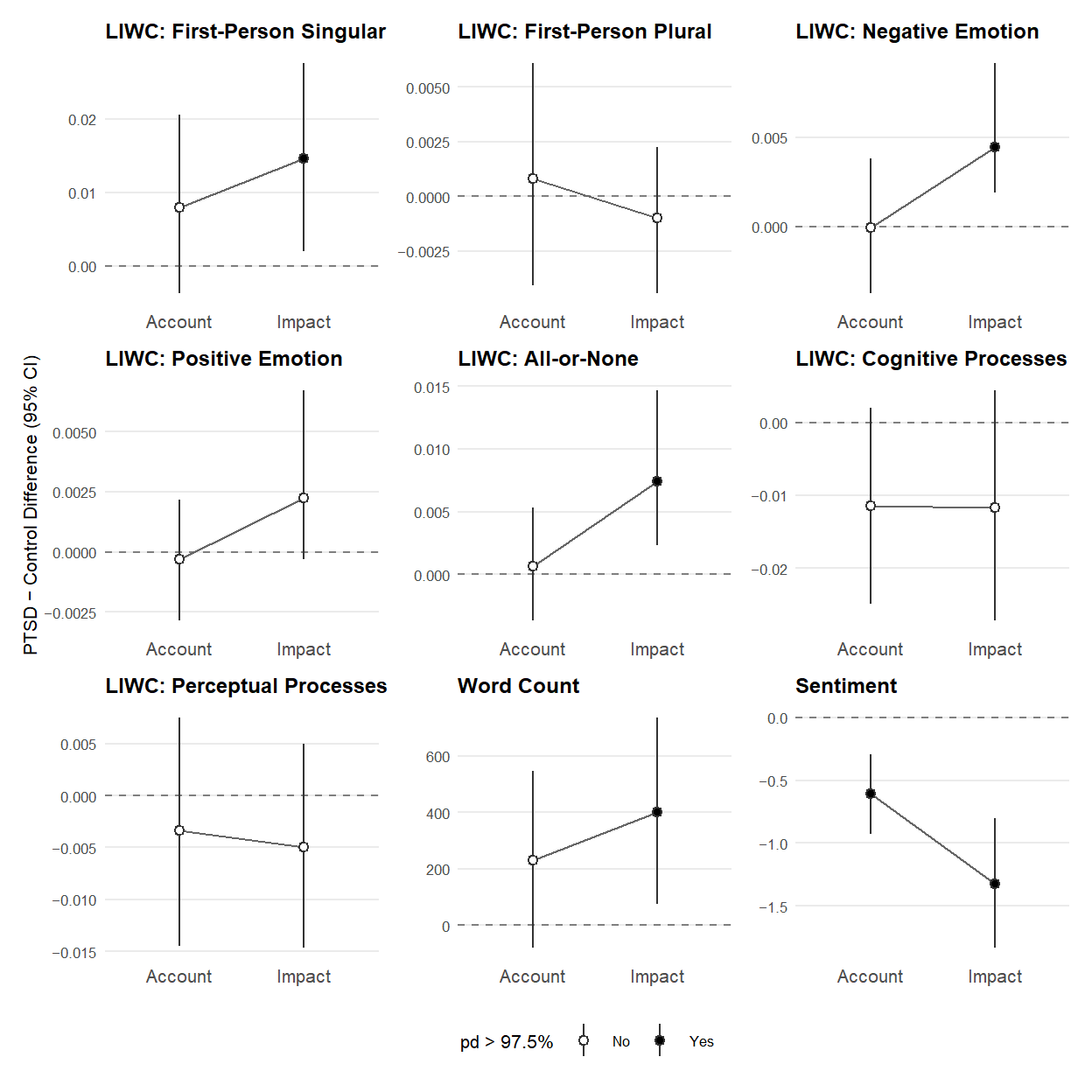
# Cairo embeds fonts and renders hyphens and minus signs correctly
ggsave("verbal.pdf", width = 6.5, height = 6.5, units = "in", device = cairo_pdf)
ggsave("verbal.png", width = 6.5, height = 6.5, units = "in", dpi = 600, device = ragg::agg_png, bg = "white")walk(
names(all_models),
\(x) {
if (x == "Sentiment") {
# performance::check_predictions() relabels ordinal draws with all six
# response levels and errors when a draw spans fewer, so use brms directly
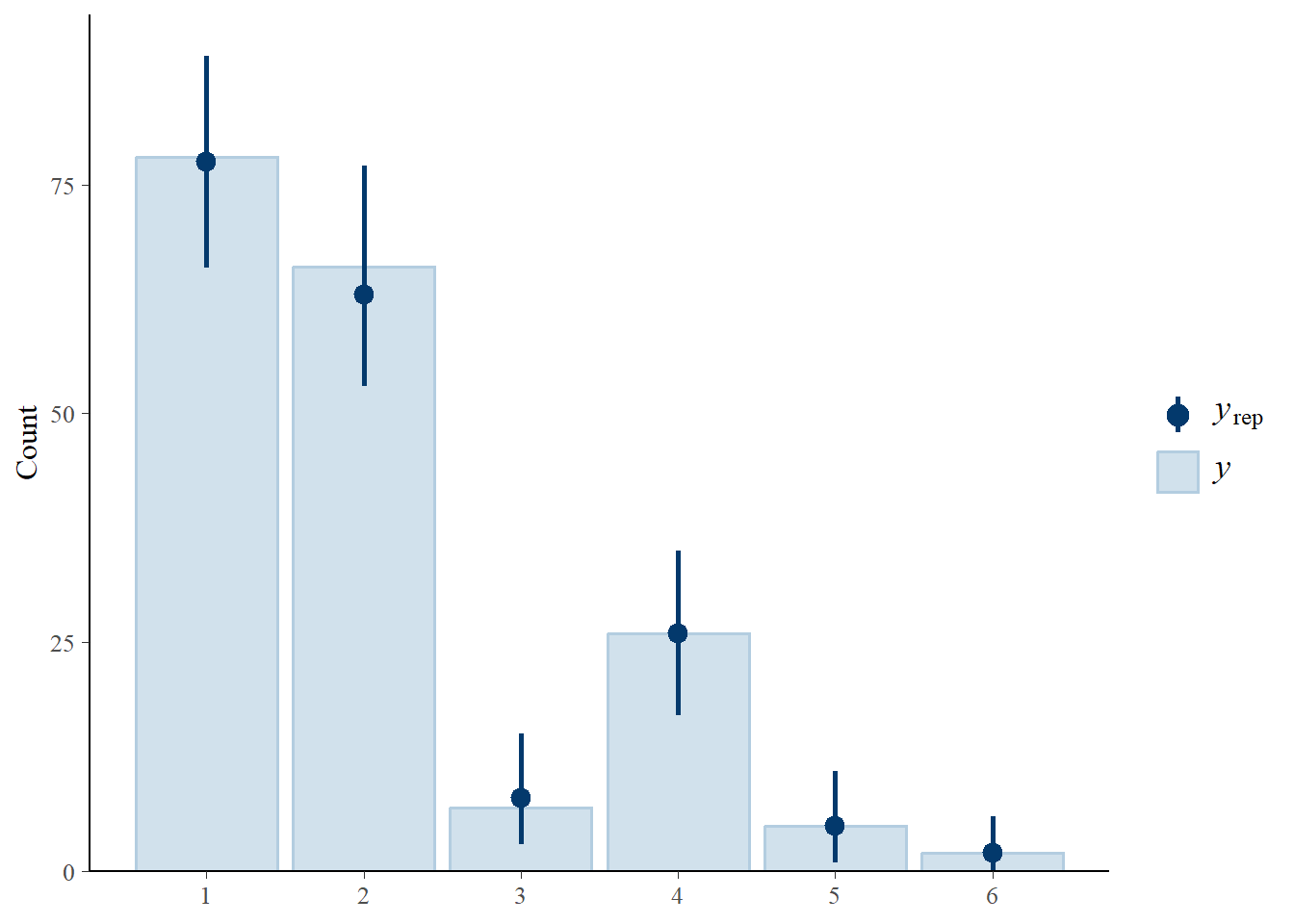
print(brms::pp_check(all_models[[x]], type = "bars", ndraws = 100))
} else {
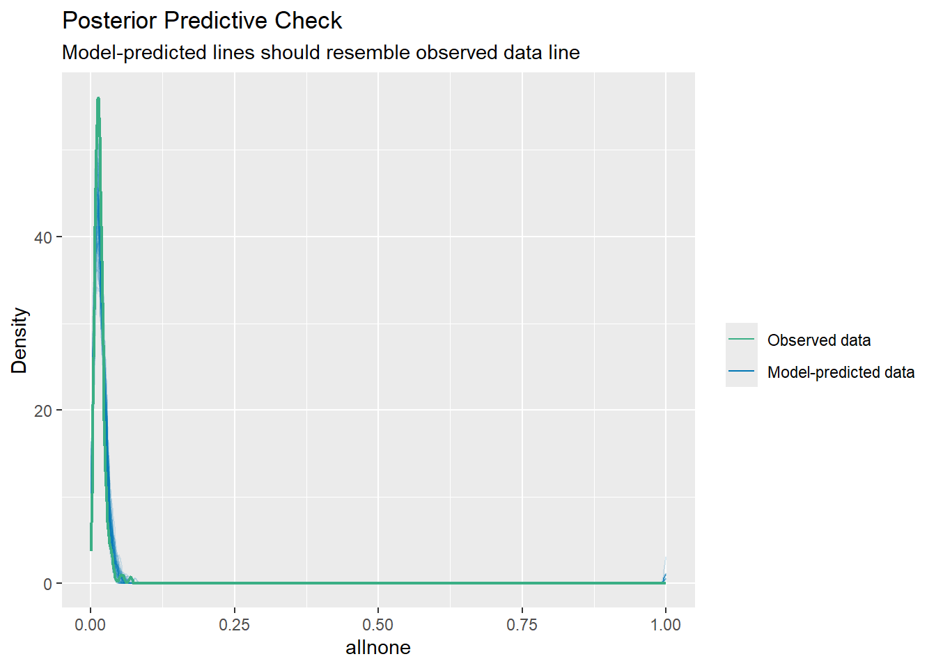
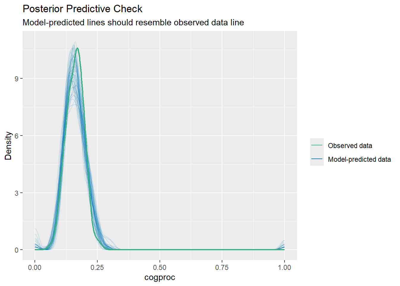
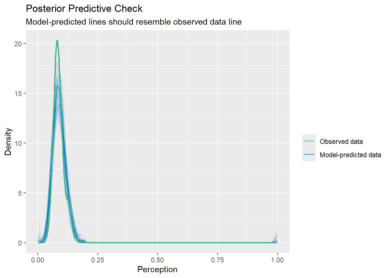
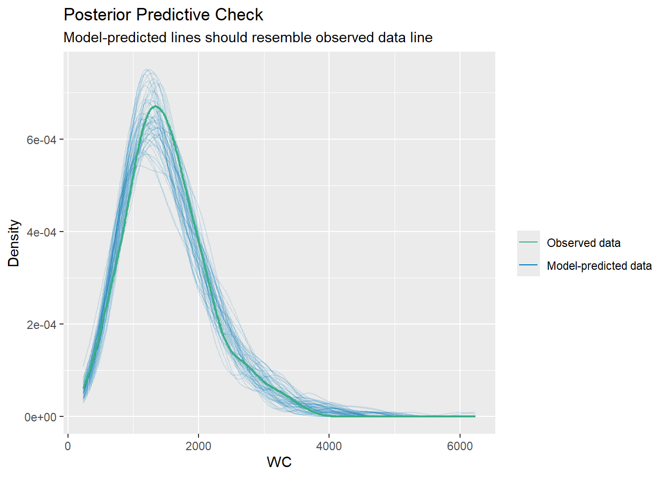
print(check_predictions(all_models[[x]], type = "density", allow_new_levels = TRUE))
}
}
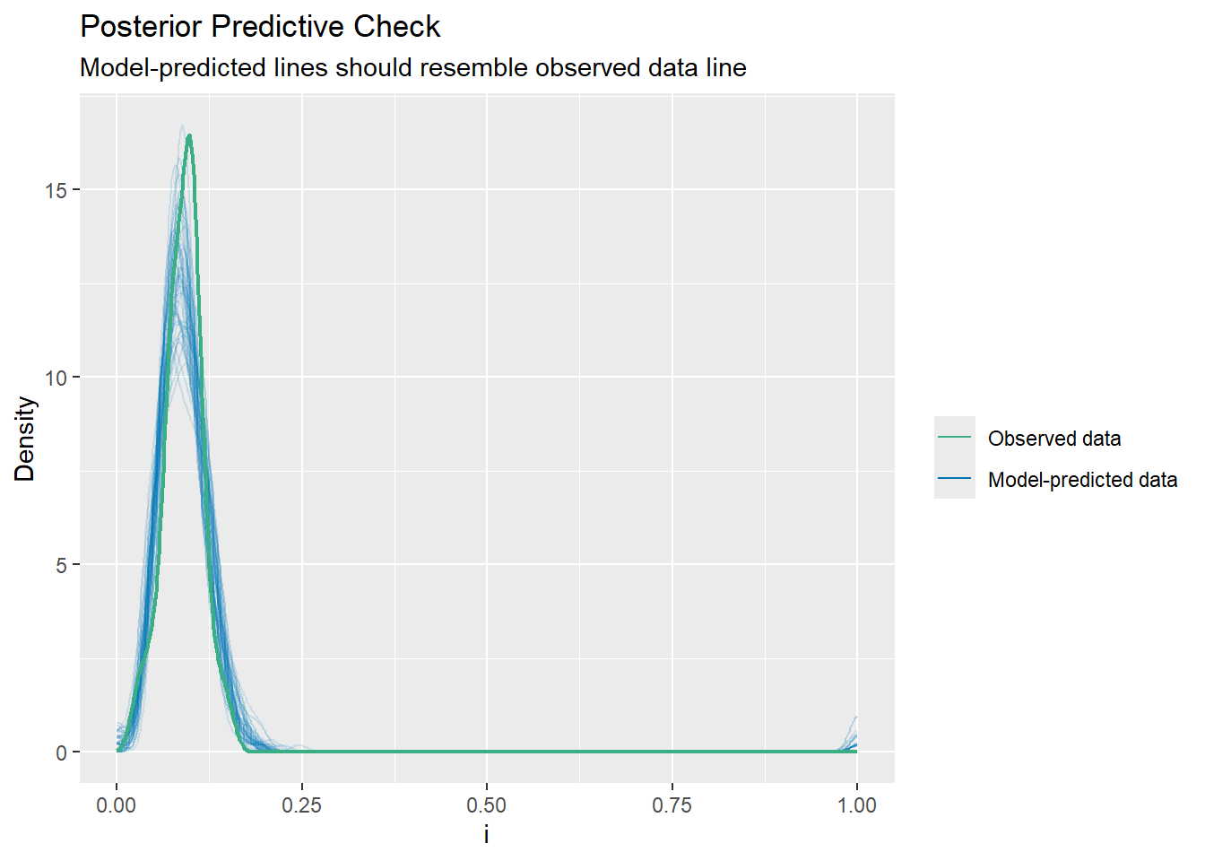
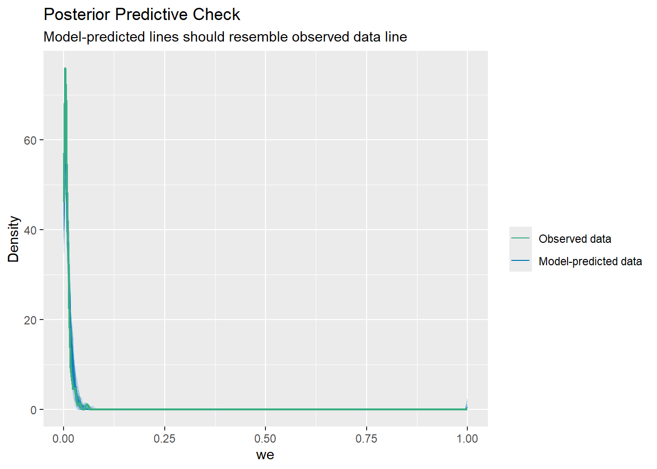
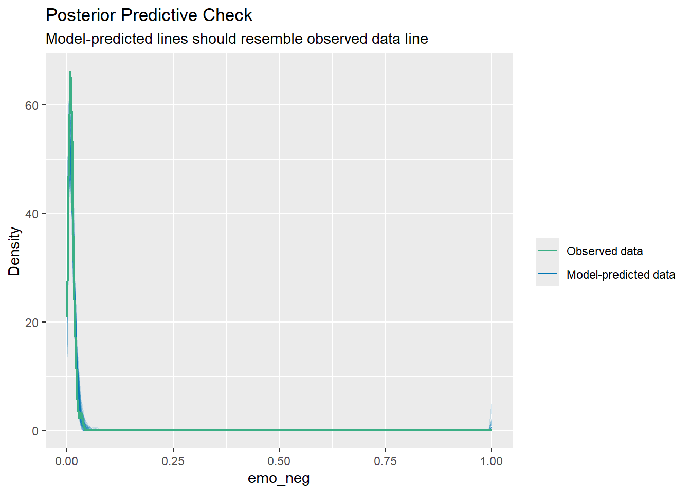
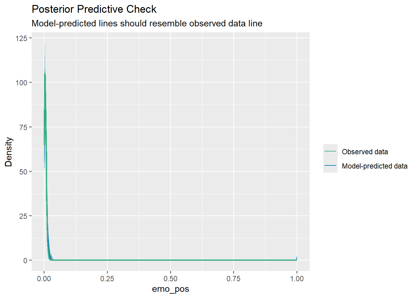
)