Visual Feature Analyses

Author

Jeffrey Girard

Published

October 5, 2026

Setup

Packages

Code

library(tidyverse)
library(easystats)
library(brms)
library(ordbetareg)
library(flextable)
library(patchwork)

Data

Code

# Deidentified features (one row per participant and task); see ../data/README.md
df_visual <-
  # base R's parser restores every stored value exactly (readr's can differ in the last digit)
  read.csv(file.path("..", "data", "visual.csv")) |>
  as_tibble() |>
  mutate(
    participant = factor(participant),
    source = factor(source, levels = c("clinic", "prolific")),
    ptsd = factor(ptsd, levels = c(0, 1)),
    demo_sex = factor(demo_sex, levels = c("Male", "Female")),
    demo_nonwhite = factor(demo_nonwhite, levels = c(FALSE, TRUE)),
    task = factor(task, levels = c("Account", "Impact")),
    # AU intensities (0-5) to proportions of the scale maximum
    AU04 = AU04 / 5, # fear, sadness, anger
    AU12 = AU12 / 5, # happiness
    AU15 = AU15 / 5, # sadness, disgust
    AU17 = AU17 / 5, # disgust
    AU20 = AU20 / 5  # fear
  ) |>
  arrange(participant, task)

# Effect-code every two-level factor (first level = -0.5, second = +0.5) so each main effect is averaged
# over the other factors (e.g., group = PTSD - Control averaged across tasks); interactions and predictions are unchanged
for (v in c("task", "ptsd", "demo_sex", "demo_nonwhite")) contrasts(df_visual[[v]]) <- c(-0.5, 0.5)
dir.create("fits", showWarnings = FALSE)

# High-ICC models whose between-person (group) coefficient mixed slowly at 4000 iterations
long_run <- c("CPPS", "H1H2", "M_Voiced", "SD_Voiced", "PoseX", "AU15")

df_visual |>
  select(AU04:DiffY) |> 
  pivot_longer(cols = everything()) |> 
  ggplot(aes(x = value)) + 
  facet_wrap(~name, scales = "free") + 
  geom_histogram(bins = 30, na.rm = TRUE)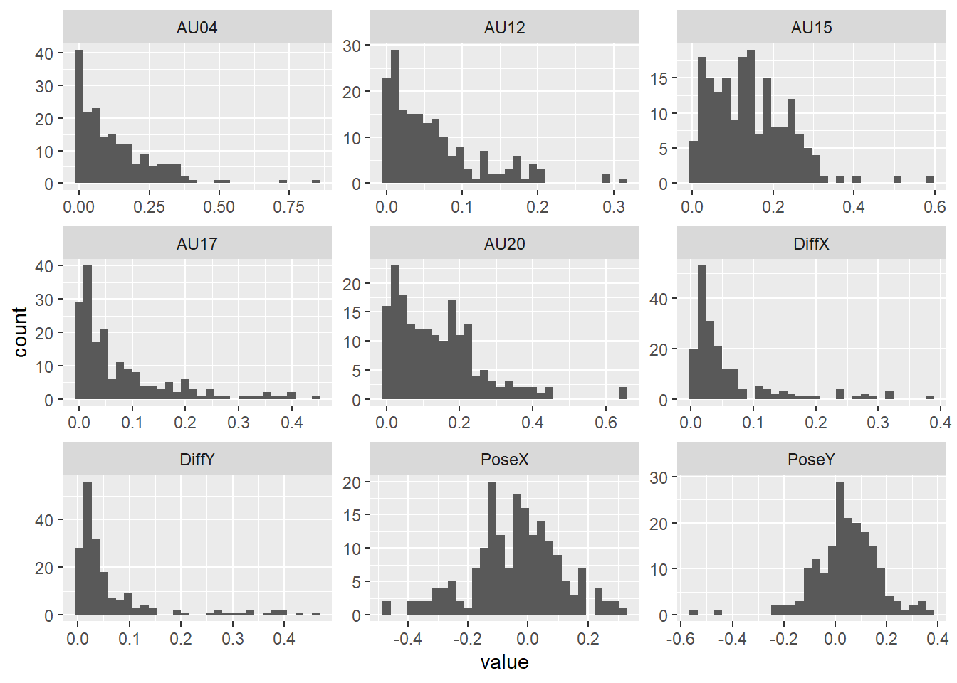

Run Models

Gaussian Models

Code

gaussian_features <- c("PoseX", "PoseY")

gaussian_models <- 
  gaussian_features |>
  set_names() |>
  map(
    \(feature) {
      model_formula <- as.formula(
        paste(feature, "~ task * ptsd + demo_age + demo_sex + demo_nonwhite + (1 | participant)")
      )
      brm(
        formula = model_formula,
        data = df_visual,
        prior = set_prior("normal(0, 1)", class = "b"),
        seed = 2026,
        chains = 4,
        cores = 4,
        iter = if (feature %in% long_run) 8000 else 4000,
        warmup = 2000,
        refresh = 0,
        file = file.path("fits", feature),
        control = list(adapt_delta = 0.95, max_treedepth = 12),
        backend = "cmdstanr"
      )
    }
  )

iwalk(
  gaussian_models,
  \(model, name) {
    thisr2 <- r2(model)
    cat(
      "\n\n#### ", 
      name, 
      sprintf("(R2C = %0.2f, R2M = %0.2f)", thisr2$R2_Bayes, thisr2$R2_Bayes_marginal),
      "\n\n"
    )
    table_md <- print_md(model_parameters(model))
    cat(table_md, sep = "\n")
  }
)

PoseX (R2C = 0.93, R2M = 0.08)

Fixed Effects
Parameter	Median	95% CI	pd	Rhat	ESS (tail)
(Intercept)	0.02	(-0.08, 0.13)	67.08%	1.002	5220
task1	3.84e-03	(-7.95e-03, 0.02)	73.95%	1.000	14875
ptsd1	-1.39e-03	(-0.08, 0.08)	51.65%	1.001	4218
demo_age	-1.91e-03	(-4.26e-03, 4.40e-04)	94.54%	1.002	4695
demo_sex1	-0.03	(-0.10, 0.04)	79.55%	1.001	4601
demo_nonwhite1	-0.06	(-0.15, 0.03)	91.12%	1.003	5371
task1:ptsd1	2.73e-03	(-0.02, 0.03)	59.24%	1.000	14907

Sigma
Parameter	Median	95% CI	pd	Rhat	ESS (tail)
sigma	0.04	(0.03, 0.05)	100%	1.000	12802

PoseY (R2C = 0.93, R2M = 0.08)

Fixed Effects
Parameter	Median	95% CI	pd	Rhat	ESS (tail)
(Intercept)	0.09	(0.02, 0.18)	99.09%	1.003	1242
task1	2.22e-03	(-7.75e-03, 0.01)	66.86%	1.000	5908
ptsd1	-3.15e-03	(-0.06, 0.06)	54.02%	1.004	1592
demo_age	-1.54e-03	(-3.57e-03, 2.34e-04)	95.55%	1.002	1281
demo_sex1	0.04	(-0.03, 0.09)	87.76%	1.005	1397
demo_nonwhite1	-0.02	(-0.10, 0.05)	72.02%	1.006	1744
task1:ptsd1	0.02	(-5.12e-03, 0.03)	93.14%	1.001	5406

Sigma
Parameter	Median	95% CI	pd	Rhat	ESS (tail)
sigma	0.03	(0.03, 0.04)	100%	1.000	4191

Inverse Gaussian Models

Code

invgaussian_features <- c("DiffX", "DiffY")

invgaussian_models <- 
  invgaussian_features |>
  set_names() |>
  map(
    \(feature) {
      model_formula <- as.formula(
        paste(feature, "~ task * ptsd + demo_age + demo_sex + demo_nonwhite + (1 | participant)")
      )
      brm(
        formula = model_formula,
        data = df_visual,
        family = inverse.gaussian(link = "log"),
        prior = set_prior("normal(0, 1)", class = "b"),
        seed = 2026,
        chains = 4,
        cores = 4,
        iter = if (feature %in% long_run) 8000 else 4000,
        warmup = 2000,
        refresh = 0,
        file = file.path("fits", feature),
        control = list(adapt_delta = 0.95, max_treedepth = 12),
        backend = "cmdstanr"
      )
    }
  )


iwalk(
  invgaussian_models,
  \(model, name) {
    thisr2 <- r2(model)
    cat(
      "\n\n#### ", 
      name, 
      sprintf("(R2C = %0.2f, R2M = %0.2f)", thisr2$R2_Bayes, thisr2$R2_Bayes_marginal),
      "\n\n"
    )
    table_md <- print_md(model_parameters(model))
    cat(table_md, sep = "\n")
  }
)

DiffX (R2C = 0.59, R2M = 0.06)

Fixed Effects
Parameter	Median	95% CI	pd	Rhat	ESS (tail)
(Intercept)	-2.63	(-3.29, -1.92)	100%	1.005	2646
task1	-0.04	(-0.18, 0.10)	71.67%	1.002	5888
ptsd1	-0.08	(-0.58, 0.40)	63.24%	1.002	2543
demo_age	-0.02	(-0.03, -2.36e-03)	98.88%	1.006	2702
demo_sex1	0.54	(0.07, 1.01)	98.76%	1.002	2393
demo_nonwhite1	-0.14	(-0.72, 0.44)	68.91%	1.002	3001
task1:ptsd1	-2.95e-03	(-0.28, 0.27)	50.90%	1.000	5757

DiffY (R2C = 0.58, R2M = 0.04)

Fixed Effects
Parameter	Median	95% CI	pd	Rhat	ESS (tail)
(Intercept)	-2.56	(-3.34, -1.75)	100%	1.002	2786
task1	0.08	(-0.08, 0.23)	83.40%	1.000	6145
ptsd1	-7.31e-03	(-0.56, 0.54)	51.05%	1.002	2985
demo_age	-0.02	(-0.04, -1.48e-03)	98.26%	1.003	2831
demo_sex1	0.48	(-0.03, 1.02)	96.66%	1.001	2786
demo_nonwhite1	-0.27	(-0.93, 0.38)	78.77%	1.001	2868
task1:ptsd1	0.05	(-0.26, 0.35)	62.31%	1.001	6011

Ordered Beta Models

Code

ob_features <- c("AU04", "AU12", "AU15", "AU17", "AU20")

ob_models <- 
  ob_features |>
  set_names() |>
  map(
    \(feature) {
      model_formula <- as.formula(
        paste(feature, "~ task * ptsd + demo_age + demo_sex + demo_nonwhite + (1 | participant)")
      )
      ordbetareg(
        formula = model_formula,
        data = df_visual,
        coef_prior_mean = 0,
        coef_prior_SD = 1,
        seed = 2026,
        chains = 4,
        cores = 4,
        iter = if (feature %in% long_run) 8000 else 4000,
        warmup = 2000,
        refresh = 0,
        file = file.path("fits", feature),
        control = list(adapt_delta = 0.95, max_treedepth = 12),
        backend = "cmdstanr"
      )
    }
  )


iwalk(
  ob_models,
  \(model, name) {
    thisr2 <- r2(model)
    cat(
      "\n\n#### ", 
      name, 
      sprintf("(R2C = %0.2f, R2M = %0.2f)", thisr2$R2_Bayes, thisr2$R2_Bayes_marginal),
      "\n\n"
    )
    table_md <- print_md(model_parameters(model))
    cat(table_md, sep = "\n")
  }
)

AU04 (R2C = 0.93, R2M = 0.13)

Fixed Effects
Parameter	Median	95% CI	pd	Rhat	ESS (tail)
(Intercept)	-4.23	(-5.16, -3.30)	100%	1.002	1429
task1	0.02	(-0.10, 0.13)	59.96%	1.000	5524
ptsd1	0.15	(-0.48, 0.77)	67.58%	1.003	1612
demo_age	0.03	(0.01, 0.06)	99.88%	1.003	1277
demo_sex1	0.44	(-0.20, 1.05)	90.44%	1.002	1530
demo_nonwhite1	-0.70	(-1.43, 0.09)	96.05%	1.004	2213
task1:ptsd1	-0.09	(-0.31, 0.15)	77.42%	1.001	5730

AU12 (R2C = 0.86, R2M = 0.04)

Fixed Effects
Parameter	Median	95% CI	pd	Rhat	ESS (tail)
(Intercept)	-3.24	(-4.03, -2.45)	100%	1.001	1982
task1	0.11	(-0.02, 0.24)	95.73%	1.000	6043
ptsd1	0.05	(-0.51, 0.61)	56.62%	1.001	2235
demo_age	5.50e-03	(-0.01, 0.02)	72.19%	1.001	2065
demo_sex1	-0.29	(-0.81, 0.23)	85.61%	1.002	2496
demo_nonwhite1	0.26	(-0.37, 0.89)	79.01%	1.004	2582
task1:ptsd1	0.20	(-0.05, 0.46)	93.73%	1.001	6443

AU15 (R2C = 0.95, R2M = 0.19)

Fixed Effects
Parameter	Median	95% CI	pd	Rhat	ESS (tail)
(Intercept)	-3.12	(-3.75, -2.50)	100%	1.001	3463
task1	0.02	(-0.04, 0.08)	73.45%	1.000	16871
ptsd1	0.56	(0.12, 0.99)	99.39%	1.002	3453
demo_age	0.03	(0.02, 0.04)	100.00%	1.003	3109
demo_sex1	-0.26	(-0.70, 0.16)	88.84%	1.002	3052
demo_nonwhite1	0.37	(-0.12, 0.89)	92.82%	1.002	3512
task1:ptsd1	-0.09	(-0.22, 0.04)	91.50%	1.000	15887

AU17 (R2C = 0.96, R2M = 0.14)

Fixed Effects
Parameter	Median	95% CI	pd	Rhat	ESS (tail)
(Intercept)	-4.34	(-5.22, -3.52)	100%	1.002	2363
task1	0.07	(-0.02, 0.16)	94.30%	1.001	5478
ptsd1	0.54	(-0.03, 1.11)	96.83%	1.004	2544
demo_age	0.03	(0.01, 0.05)	99.95%	1.002	1696
demo_sex1	-1.06	(-1.62, -0.47)	99.98%	1.003	1919
demo_nonwhite1	-0.11	(-0.79, 0.60)	62.99%	1.003	2625
task1:ptsd1	0.07	(-0.10, 0.24)	79.95%	1.000	4921

AU20 (R2C = 0.92, R2M = 0.08)

Fixed Effects
Parameter	Median	95% CI	pd	Rhat	ESS (tail)
(Intercept)	-3.07	(-3.88, -2.23)	100%	1.012	1336
task1	-0.04	(-0.13, 0.06)	77.69%	1.001	5108
ptsd1	0.07	(-0.52, 0.65)	59.59%	1.006	1473
demo_age	0.02	(2.71e-03, 0.04)	98.72%	1.014	1336
demo_sex1	0.19	(-0.37, 0.75)	74.95%	1.004	1683
demo_nonwhite1	0.37	(-0.35, 1.04)	85.22%	1.003	1365
task1:ptsd1	-0.03	(-0.23, 0.16)	63.36%	1.000	5628

Results Tables

Code

all_models <- c(gaussian_models, invgaussian_models, ob_models)

extract_model_stats <- function(model, model_name) {
  describe_posterior(model, effects = "fixed", component = "conditional", test = "pd") |>
    as_tibble() |>
    filter(str_detect(Parameter, "task|ptsd")) |>
    mutate(
      stars = case_when(
        pd >= 0.995 ~ "***",
        pd >= 0.985 ~ "**",
        pd >= 0.975 ~ "*",
        TRUE        ~ ""
      ),
      formatted_stat = sprintf("%.2f [%.2f, %.2f]%s", Median, CI_low, CI_high, stars),
      
      Term = case_when(
        str_detect(Parameter, ":") ~ "Interaction",
        str_detect(Parameter, "task") ~ "Main_Task",
        str_detect(Parameter, "ptsd") ~ "Main_PTSD",
        TRUE ~ Parameter
      )
    ) |>
    select(Term, formatted_stat) |>
    pivot_wider(names_from = Term, values_from = formatted_stat) |>
    mutate(Feature = model_name, .before = 1)
}

table_data <- imap(all_models, \(model, name) extract_model_stats(model, name)) |>
  list_rbind()

final_table <- 
  flextable(table_data) |>
  set_header_labels(
    Feature = "Feature",
    Main_Task = "Main Effect: Task",
    Main_PTSD = "Main Effect: PTSD",
    Interaction = "Task × PTSD Effect"
  ) |>
  autofit() |>
  add_footer_lines("Note: Estimates are median posterior values on the link scale (identity, log, or logit). Models control for age, sex, and race. Brackets indicate 95% Credible Intervals. * pd > 97.5%, ** pd > 98.5%, *** pd > 99.5%. ")

final_table

Feature	Main Effect: Task	Main Effect: PTSD	Task × PTSD Effect
PoseX	0.00 [-0.01, 0.02]	-0.00 [-0.08, 0.08]	0.00 [-0.02, 0.03]
PoseY	0.00 [-0.01, 0.01]	-0.00 [-0.06, 0.06]	0.02 [-0.01, 0.03]
DiffX	-0.04 [-0.18, 0.10]	-0.08 [-0.58, 0.40]	-0.00 [-0.28, 0.27]
DiffY	0.08 [-0.08, 0.23]	-0.01 [-0.56, 0.54]	0.05 [-0.26, 0.35]
AU04	0.02 [-0.10, 0.13]	0.15 [-0.48, 0.77]	-0.09 [-0.31, 0.15]
AU12	0.11 [-0.02, 0.24]	0.05 [-0.51, 0.61]	0.20 [-0.05, 0.46]
AU15	0.02 [-0.04, 0.08]	0.56 [0.12, 0.99]**	-0.09 [-0.22, 0.04]
AU17	0.07 [-0.02, 0.16]	0.54 [-0.03, 1.11]	0.07 [-0.10, 0.24]
AU20	-0.04 [-0.13, 0.06]	0.07 [-0.52, 0.65]	-0.03 [-0.23, 0.16]
Note: Estimates are median posterior values on the link scale (identity, log, or logit). Models control for age, sex, and race. Brackets indicate 95% Credible Intervals. * pd > 97.5%, pd > 98.5%, * pd > 99.5%.

Code

# Simple group effects (PTSD - Control) within each task on the response scale,
# averaged over sex and race (equal weights, matching the effect coding) at the
# mean age, with random intercepts at zero
extract_group_deltas <- function(model, model_name) {
  ec <- estimate_contrasts(model, contrast = "ptsd", by = "task", re_formula = NA) |>
    as.data.frame()
  stopifnot(all(ec$Level1 == "1" & ec$Level2 == "0"))  # PTSD minus Control
  ec |>
    transmute(
      Feature = model_name,
      Task = as.character(task),
      Estimate = Median,
      CI_Low = CI_low,
      CI_High = CI_high,
      pd
    )
}

group_delta_results <- imap(all_models, \(model, name) {
  extract_group_deltas(model, name)
}) |> list_rbind()

group_delta_table <- 
  group_delta_results |>
  mutate(Feature = gsub("_", " ", Feature)) |>
  flextable() |>
  colformat_double(
    j = c("Estimate", "CI_Low", "CI_High"), 
    digits = 3
  ) |>
  colformat_double(
    j = "pd", 
    digits = 3
  ) |>
  set_header_labels(
    Feature = "Feature",
    Task = "Task",
    Estimate = "PTSD Δ", # PTSD minus Control
    CI_Low = "Lower 95% CI",
    CI_High = "Upper 95% CI",
    pd = "pd"
  ) |>
  autofit() |>
  italic(j = "pd", part = "header") |>
  bold(i = ~ pd > 0.975, j = c("Estimate", "pd")) |>
  add_footer_lines("Note: PTSD Δ is the estimated difference (PTSD - Control) on the response scale, averaged over sex and race at the mean age. pd = Probability of Direction. Bold rows indicate pd > 0.975.")

group_delta_table

Feature	Task	PTSD Δ	Lower 95% CI	Upper 95% CI	pd
PoseX	Account	-0.003	-0.079	0.075	0.529
PoseX	Impact	-0.000	-0.076	0.078	0.503
PoseY	Account	-0.011	-0.071	0.052	0.635
PoseY	Impact	0.005	-0.056	0.068	0.553
DiffX	Account	-0.003	-0.024	0.016	0.624
DiffX	Impact	-0.003	-0.023	0.016	0.631
DiffY	Account	-0.001	-0.022	0.020	0.546
DiffY	Impact	0.001	-0.022	0.025	0.523
AU04	Account	0.011	-0.026	0.052	0.715
AU04	Impact	0.006	-0.031	0.046	0.627
AU12	Account	-0.002	-0.030	0.026	0.572
AU12	Impact	0.007	-0.021	0.040	0.698
AU15	Account	0.070	0.018	0.130	0.996
AU15	Impact	0.061	0.009	0.120	0.989
AU17	Account	0.026	-0.004	0.070	0.958
AU17	Impact	0.032	0.000	0.079	0.975
AU20	Account	0.008	-0.051	0.069	0.614
AU20	Impact	0.005	-0.052	0.065	0.573
Note: PTSD Δ is the estimated difference (PTSD - Control) on the response scale, averaged over sex and race at the mean age. pd = Probability of Direction. Bold rows indicate pd > 0.975.

Results Figures

Code

plot_titles <- c(
  "Pose: Vertical (Pitch)",
  "Pose: Horizontal (Yaw)",
  "Motion: Vertical (Pitch)",
  "Motion: Horizontal (Yaw)",
  "AU04: Brow lowerer",
  "AU12: Lip corner puller",
  "AU15: Lip corner depressor",
  "AU17: Chin raiser",
  "AU20: Mouth stretcher"
)

# Plot the simple group effects from the table above: PTSD minus Control within
# each task, with 95% credible intervals; filled points have pd > 97.5%
make_model_plot <- function(name, title) {
  d <- group_delta_results |>
    filter(Feature == name) |>
    mutate(
      Task = factor(Task, levels = c("Account", "Impact")),
      credible = factor(pd > 0.975, levels = c(FALSE, TRUE), labels = c("No", "Yes"))
    )
  ggplot(d, aes(x = Task, y = Estimate, group = 1)) +
    geom_hline(yintercept = 0, linetype = "dashed", color = "grey50") +
    geom_line(color = "grey40") +
    geom_pointrange(
      aes(ymin = CI_Low, ymax = CI_High, fill = credible),
      shape = 21, size = 0.4, color = "grey20", show.legend = TRUE
    ) +
    scale_fill_manual(values = c(No = "white", Yes = "black"), limits = c("No", "Yes"), drop = FALSE) +
    # typographic minus signs on the y-axis (Cairo otherwise draws a hyphen)
    scale_y_continuous(labels = \(x) sub("^-", "\u2212", format(x, trim = TRUE))) +
    labs(title = title, x = NULL, y = "PTSD − Control Difference (95% CI)", fill = "pd > 97.5%") +
    theme_minimal(base_size = 8) +
    theme(
      plot.title = element_text(size = 9, face = "bold"),
      axis.text.x = element_text(size = 8),
      panel.grid.minor = element_blank(),
      panel.grid.major.x = element_blank()
    )
}

plot_list <- map2(names(all_models), plot_titles, make_model_plot)

combined_plot <- wrap_plots(plot_list, ncol = 3) +
  plot_layout(guides = "collect", axis_titles = "collect") &
  theme(legend.position = "bottom")

combined_plot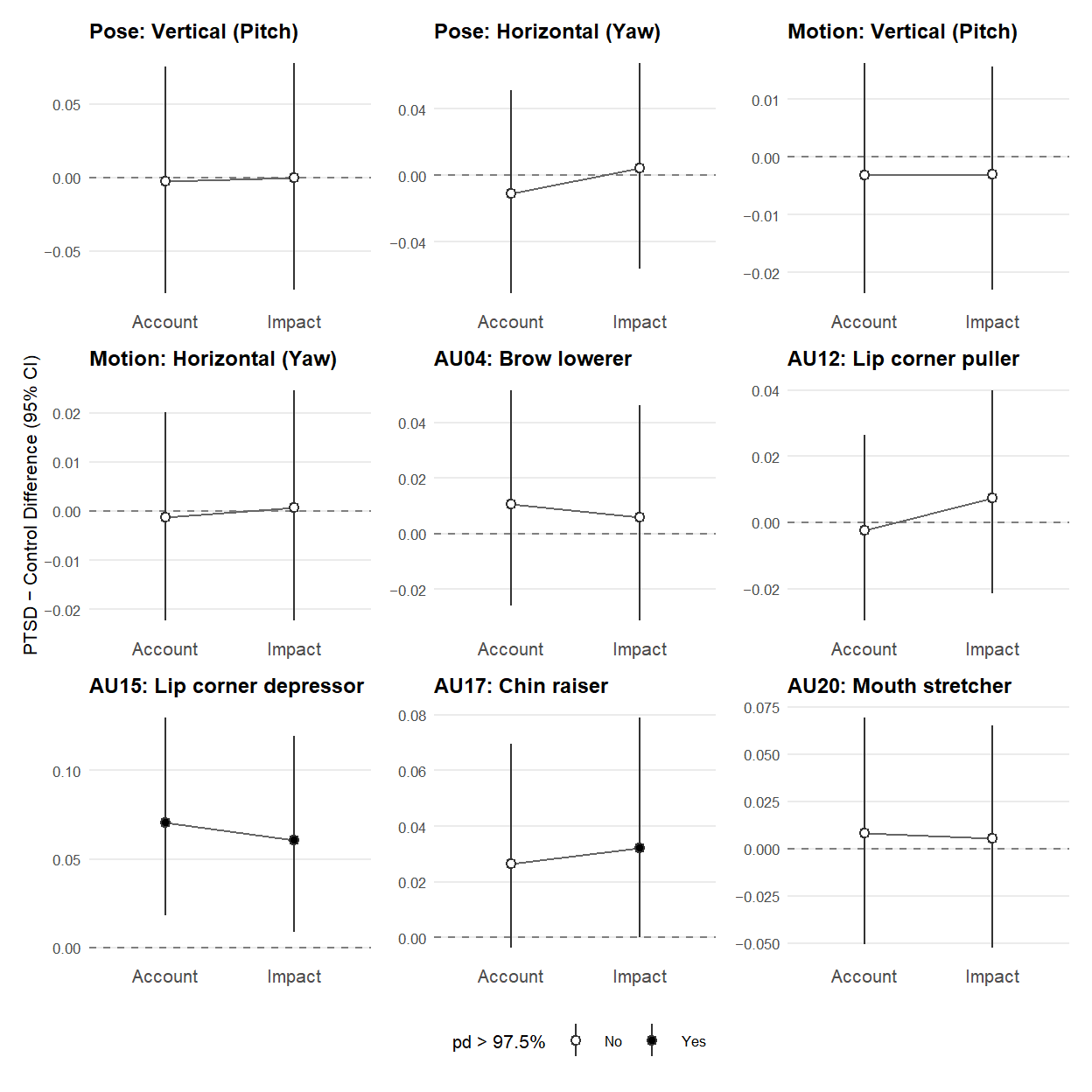

Code

# Cairo embeds fonts and renders hyphens and minus signs correctly
ggsave("visual.pdf", width = 6.5, height = 6.5, units = "in", device = cairo_pdf)
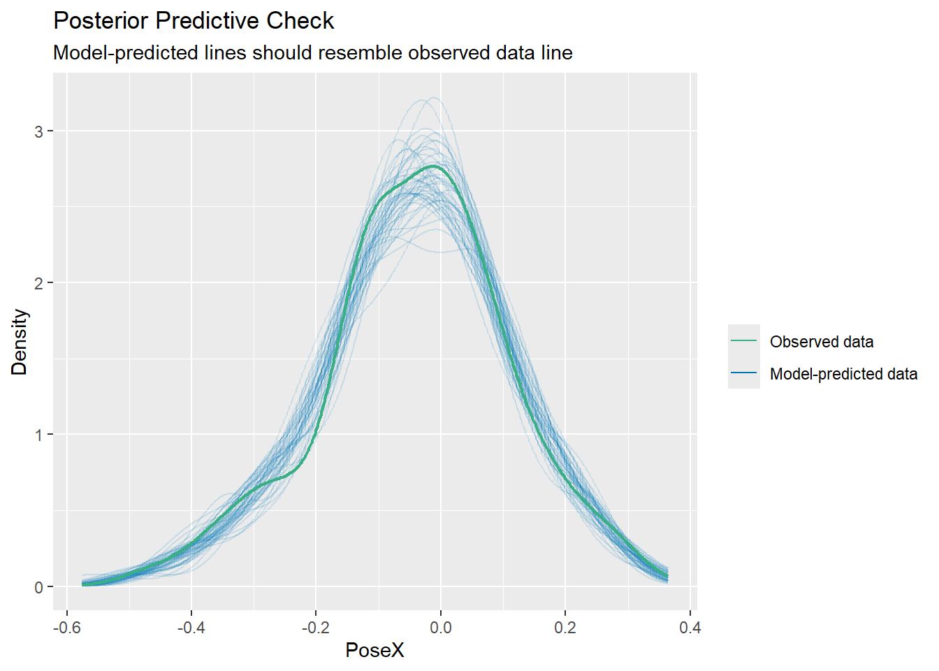
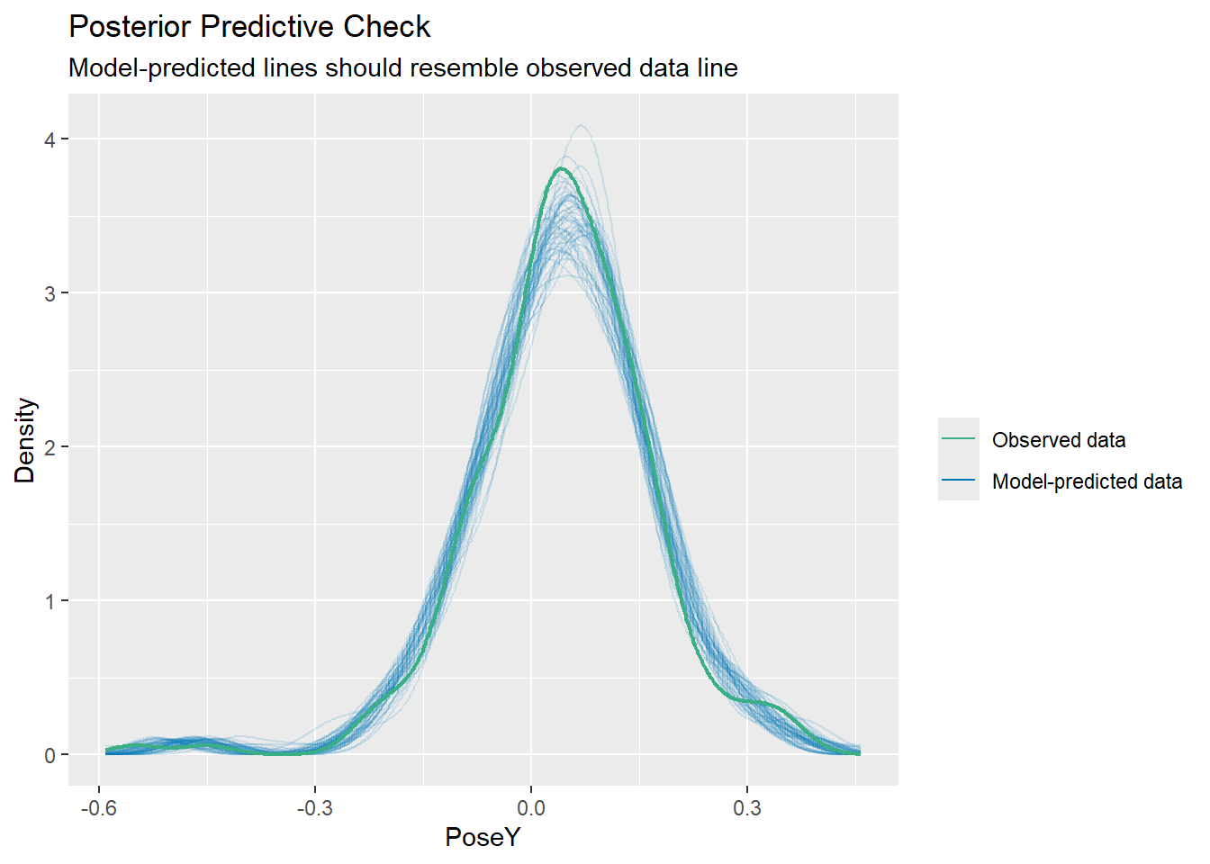
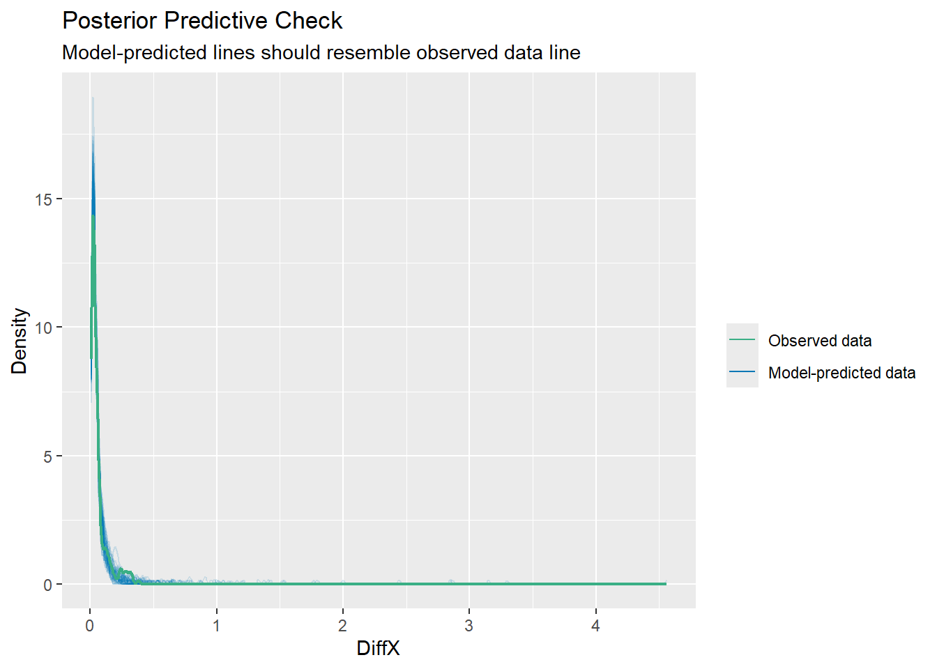
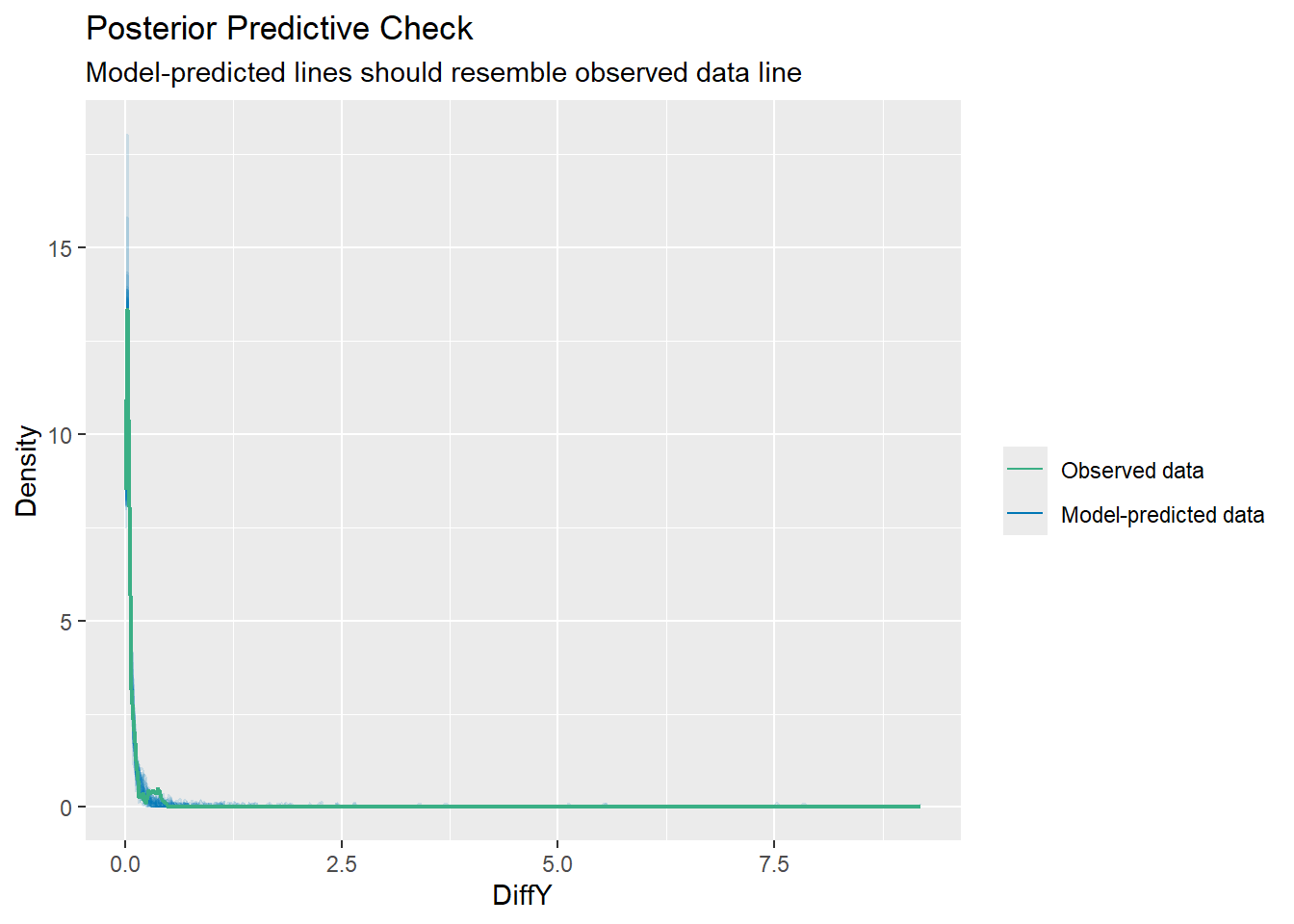
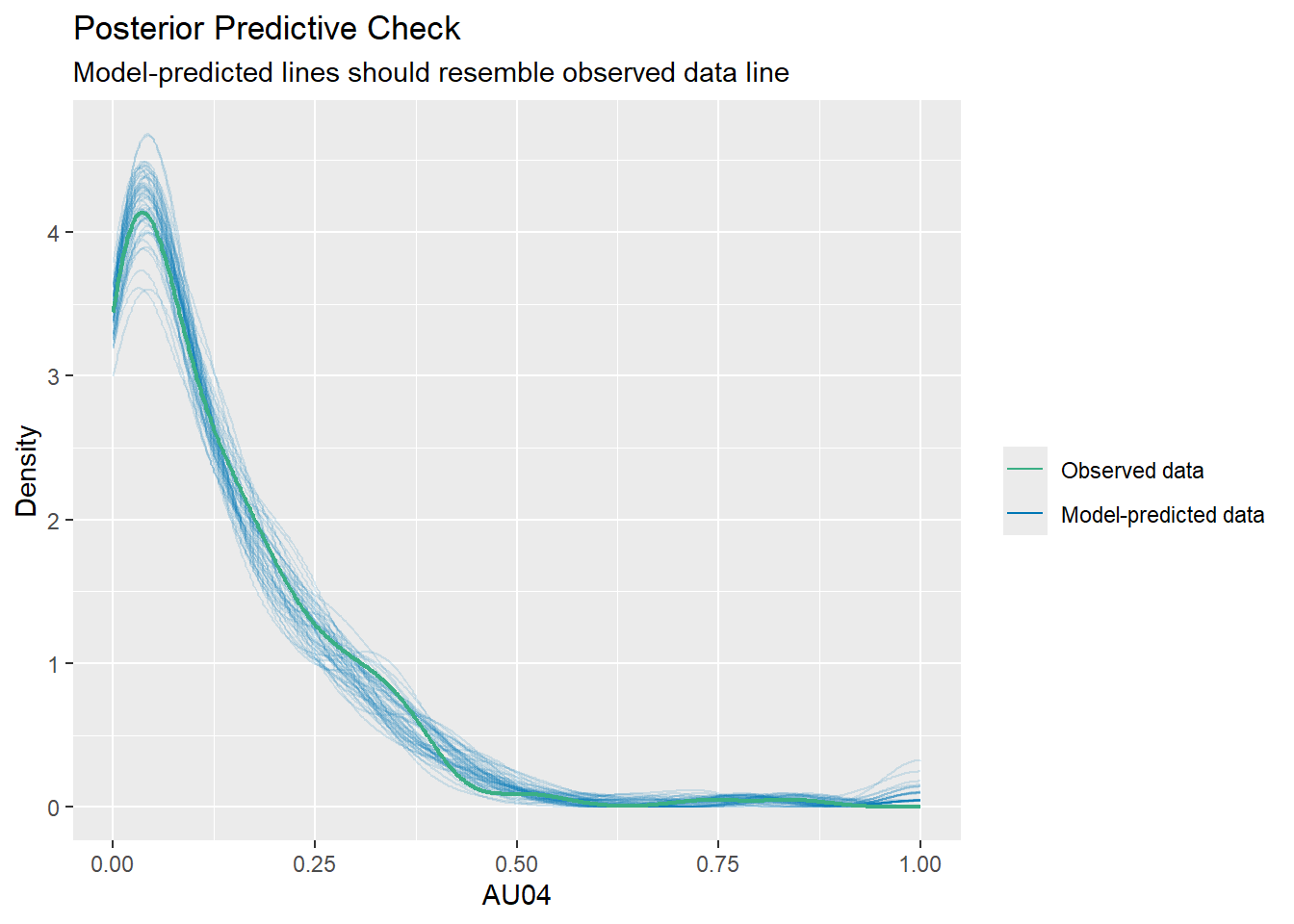
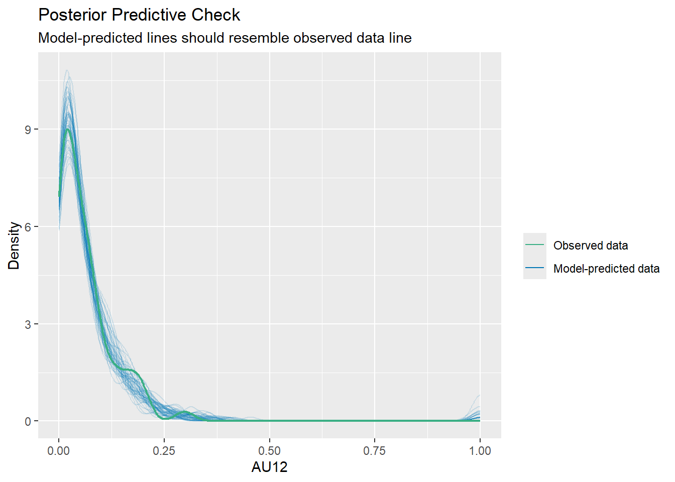
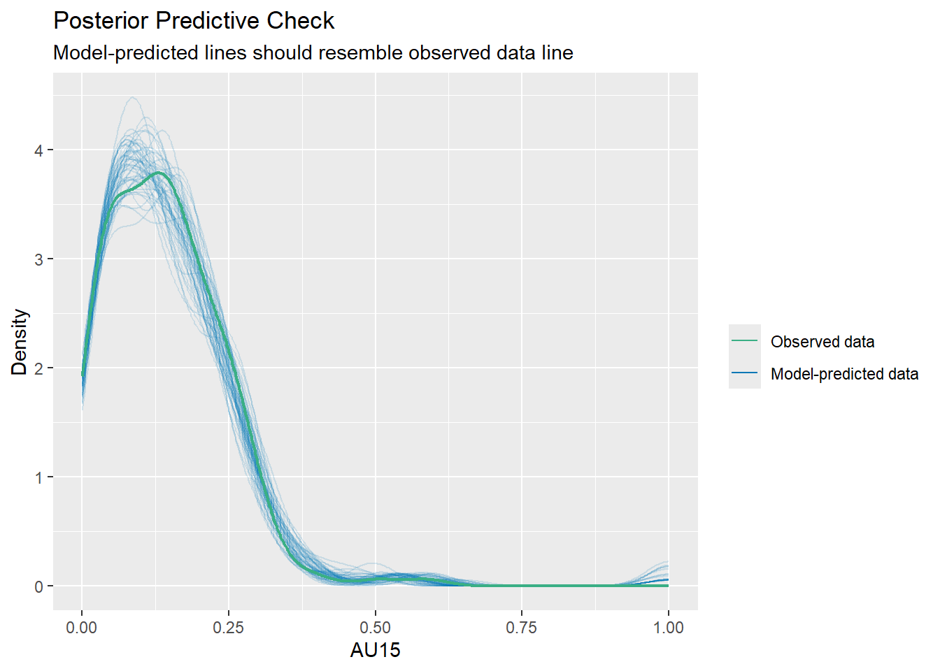
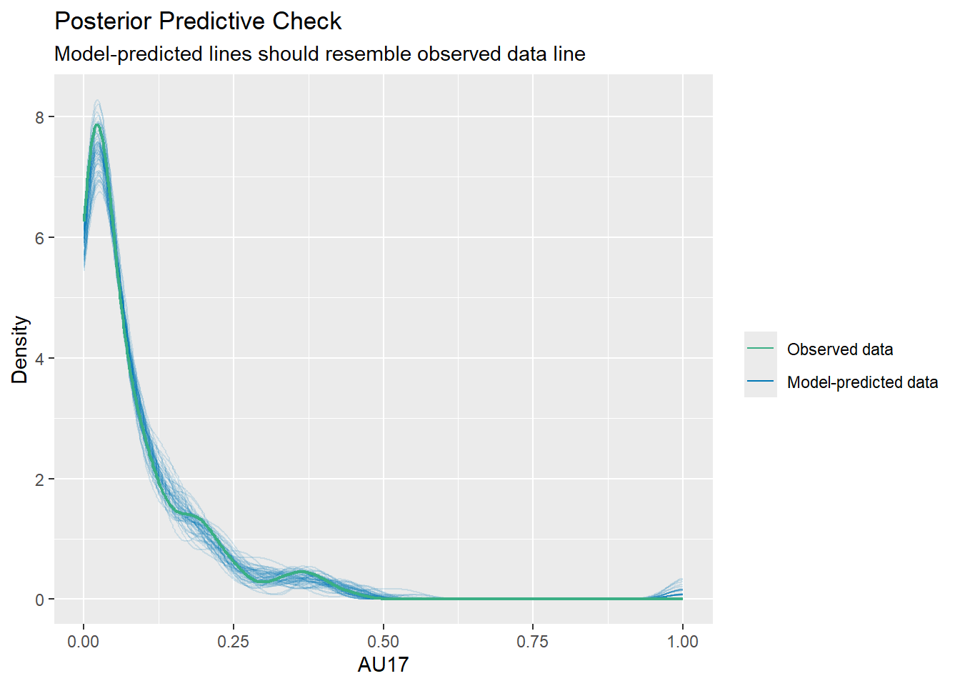
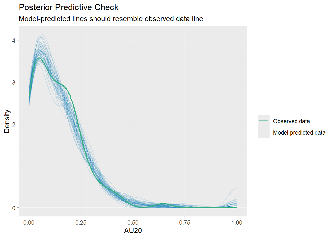
ggsave("visual.png", width = 6.5, height = 6.5, units = "in", dpi = 600, device = ragg::agg_png, bg = "white")

Diagnostics

Click to show figures

Code

walk(all_models, \(x) print(check_predictions(x, type = "density", allow_new_levels = TRUE)))