Multilevel Modeling

Linear Modeling Review (2/2)

Spring 2026 | CLAS | PSYC 894
Jeffrey M. Girard | Lecture 02b

Roadmap

1. Continous-by-Continous
   Variable Moderation

2. Continuous-by-Discrete
   Variable Moderation

3. Assumptions, Diagnostics,
   and Extensions of LM

Setup

library(easystats)
library(ggplot2)
library(marginaleffects)
library(qqplotr)
library(sandwich)

data("penguins", "mtcars", "cars", "airquality")

theme_set(theme_bw(base_size = 20))

New Packages:

• qqplotr is called by easystats to add CIs to diagnostic plots
• sandwich is called by easystats to implement HC3 corrections

Moderation

• We may want to know if the effect of one predictor depends on the value on another predictor

• To answer these, we can test interaction effects
  • Interaction effects are just slopes for the product of two or more predictors
  • Centering continous predictors is helpful

• Types of bivariate moderation
  • Continuous-by-Continuous Moderation (CCM)
  • Continuous-by-Discrete Moderation (CDM)
  • Discrete-by-Discrete Moderation (DDM)
  • Higher-order (e.g., three-way) Moderation

CCM

Continuous-by-Continuous Moderation

CCM Equation

Generic

\[y_i = \beta_0 + \beta_1 x_{1i} + \beta_2 x_{2i} + \beta_3 (x_{1i} x_{2i}) + \varepsilon_{i}\]

Example

\[\text{MASS}_i = \beta_0 + \beta_1 \text{FLEN}_{i} + \beta_2 \text{BDEP}_{i} + \\ \beta_3 \text{FLEN}_i \text{BDEP}_i + \varepsilon_i\]

CCM Formula

Generic

y ~ 1 + x1 * x2

Example

body_mass ~ 1 + flipper_len * bill_dep

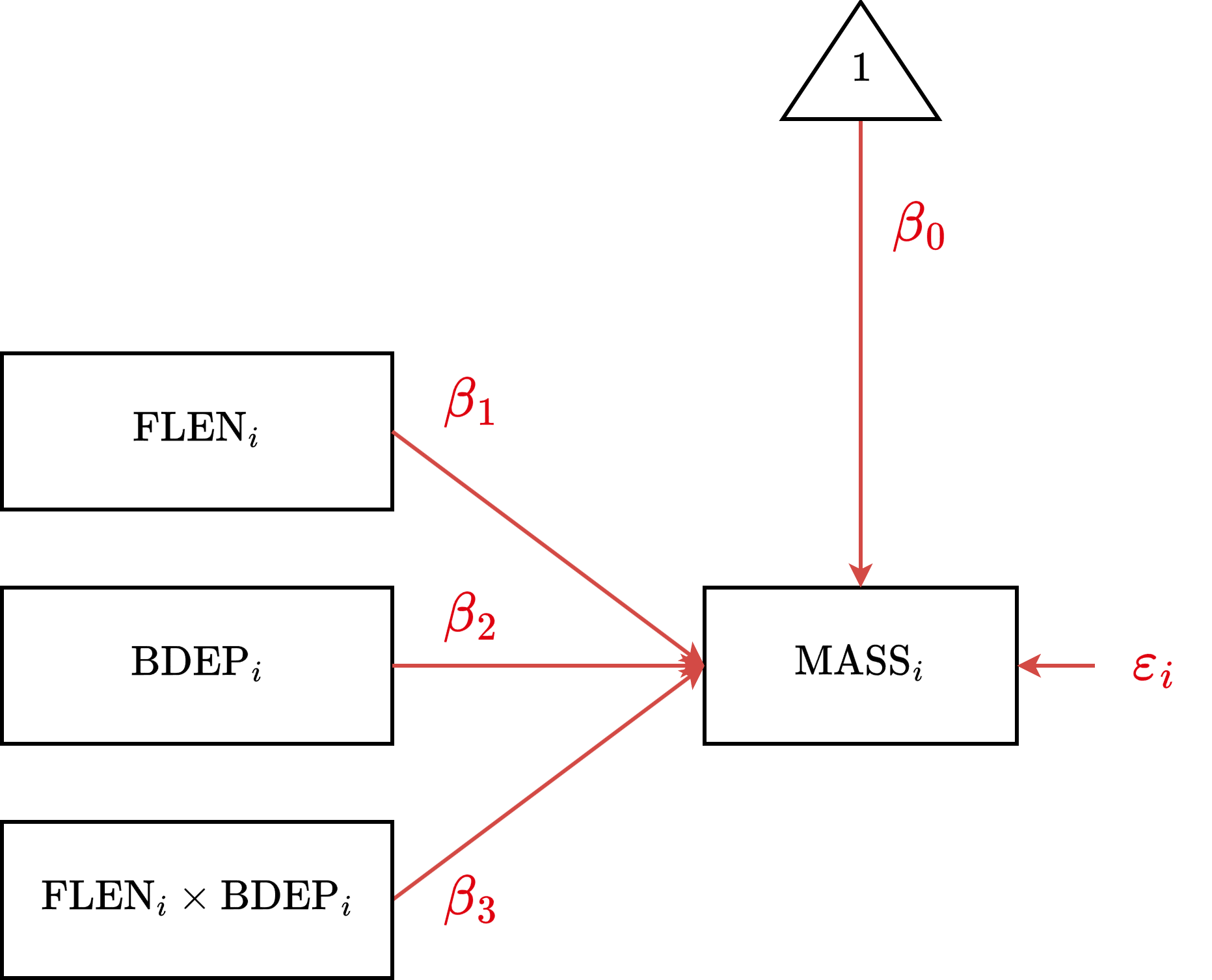
CCM Diagram

CCM Estimation

penguins_c <- center(penguins, select = c("flipper_len", "bill_dep"))
ccm_fb <- lm(
  formula = body_mass ~ 1 + flipper_len * bill_dep,
  data = penguins_c
)

model_parameters(ccm_fb)

Parameter              | Coefficient |    SE |             95% CI | t(338) |      p
-----------------------------------------------------------------------------------
(Intercept)            |     4062.79 | 29.56 | [4004.65, 4120.93] | 137.46 | < .001
flipper len            |       48.63 |  1.82 | [  45.05,   52.22] |  26.71 | < .001
bill dep               |       44.64 | 13.02 | [  19.04,   70.25] |   3.43 | < .001
flipper len × bill dep |       -8.60 |  1.34 | [ -11.23,   -5.96] |  -6.41 | < .001

CCM Interpretation

After centering the flipper length and bill depth predictors, …

• Intercept \((\beta_0=4063.8\), \(p<.001)\)
  The expected body mass for a penguin with average flipper length and bill depth.

• Flipper Length Simple Effect \((\beta_1=48.6\), \(p<.001)\)
  The expected change in body mass associated with an increase of 1mm flipper length,
  specifically for a penguin with average bill depth.

• Bill Depth Simple Effect \((\beta_2=44.6\), \(p<.001)\)
  The expected change in body mass associated with an increase of 1mm bill depth,
  specifically for a penguin with average flipper length.

• Flipper-Length-by-Bill-Depth Interaction Effect \((\beta_3=-8.6\), \(p<.001)\)
  The expected change in the slope of one predictor for an increase of 1 in the other.
  The negative sign here means the flipper length effect gets weaker as bills get deeper.

CCM Visualization 1

pred_ccmf <- estimate_relation(
  model = ccm_fb, 
  by = c(
    "flipper_len", 
    "bill_dep = [quartiles]"
  ), 
  estimate = "average"
)

plot(pred_ccmf) +
  labs(
    x = "Flipper Length", 
    y = "Body Mass", 
    color = "Bill Depth", 
    fill = "Bill Depth"
  ) +
  theme(legend.position = "top")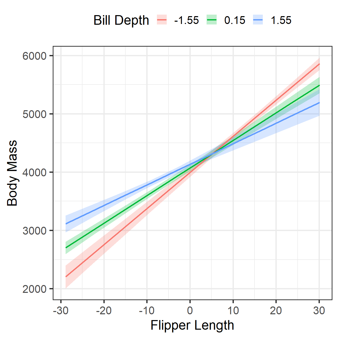

CCM Visualization 2

pred_ccmb <- estimate_relation(
  model = ccm_fb, 
  by = c(
    "bill_dep", 
    "flipper_len = [quartiles]"
  ), 
  estimate = "average"
)

plot(pred_ccmb) +
  labs(
    x = "Bill Depth", 
    y = "Body Mass", 
    color = "Flipper Length", 
    fill = "Flipper Length"
  ) +
  theme(legend.position = "top")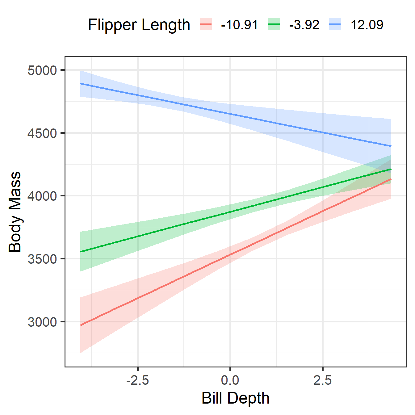

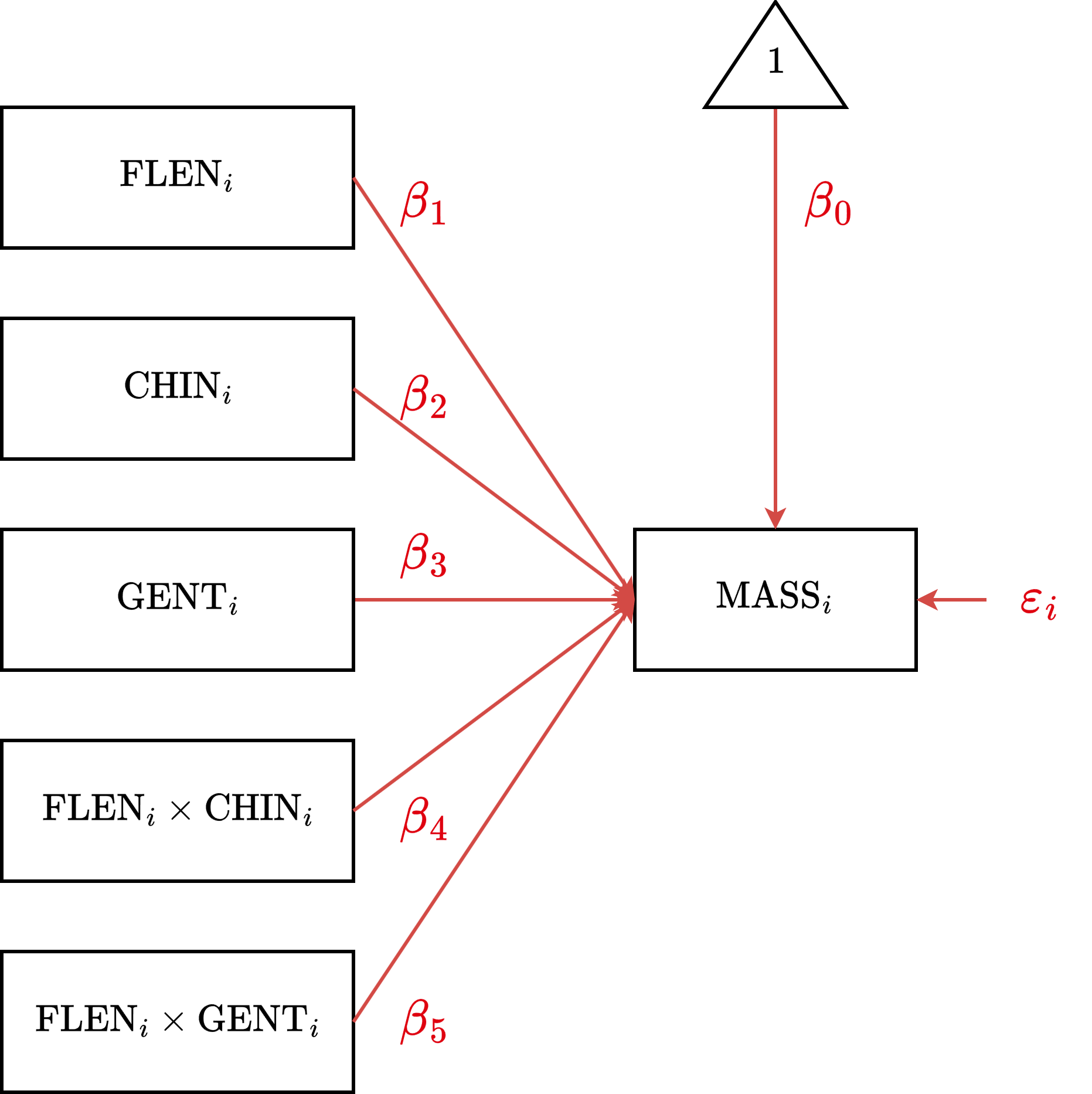
CCM Simple Slopes 1

estimate_slopes(
  model = ccm_fb, 
  trend = "flipper_len", 
  by = "bill_dep = [quartiles]"
)

Estimated Marginal Effects

bill_dep | Slope |   SE |         95% CI | t(338) |      p
----------------------------------------------------------
-1.55    | 61.97 | 2.40 | [57.25, 66.69] |  25.84 | < .001
0.15     | 47.35 | 1.88 | [43.65, 51.05] |  25.18 | < .001
1.55     | 35.32 | 3.08 | [29.25, 41.38] |  11.45 | < .001

Marginal effects estimated for flipper_len
Type of slope was dY/dX

CCM Simple Slopes 2

estimate_slopes(
  model = ccm_fb, 
  trend = "bill_dep", 
  by = "flipper_len = [quartiles]"
)

Estimated Marginal Effects

flipper_len |  Slope |    SE |           95% CI | t(338) |      p
-----------------------------------------------------------------
-10.91      | 138.47 | 22.01 | [ 95.17, 181.77] |   6.29 | < .001
-3.92       |  78.30 | 15.28 | [ 48.25, 108.34] |   5.13 | < .001
12.09       | -59.25 | 17.90 | [-94.46, -24.03] |  -3.31 |  0.001

Marginal effects estimated for bill_dep
Type of slope was dY/dX

CDM

Continuous-by-Discrete Moderation

CDM Equation

Generic

\[ \begin{aligned} y_i &= \overbrace{(\beta_0 + \beta_2 D_{1i} + \dots)}^{\text{Group-Specific Intercept}} + \overbrace{(\beta_1 + \beta_3 D_{1i} + \dots)}^{\text{Group-Specific Slope}} \cdot x_i + \varepsilon_i \end{aligned} \]

Example

\[ \begin{aligned} \text{MASS}_i &= (\beta_0 + \beta_2 \text{CHIN}_{i} + \beta_3 \text{GENT}_i) \\ &\quad + (\beta_1 + \beta_4 \text{CHIN}_{i} + \beta_5 \text{GENT}_i) \cdot \text{FLEN}_i + \varepsilon_i \end{aligned} \]

CDM Formula

Generic

y ~ 1 + x * f

Example

mass ~ 1 + flipper * species

CDM Diagram

CDM Estimation

penguins_c <- center(penguins, select = "flipper_len")
cdm_fs <- lm(
  formula = body_mass ~ 1 + flipper_len * species, 
  data = penguins_c
)

model_parameters(cdm_fs) |> print(select = "minimal")

Parameter                         | Coefficient |             95% CI |      p
-----------------------------------------------------------------------------
(Intercept)                       |     4060.55 | [3944.47, 4176.62] | < .001
flipper len                       |       32.83 | [  23.73,   41.93] | < .001
species [Chinstrap]               |     -151.42 | [-310.58,    7.73] | 0.062 
species [Gentoo]                  |      126.66 | [ -85.98,  339.31] | 0.242 
flipper len × species [Chinstrap] |        1.74 | [ -13.71,   17.19] | 0.825 
flipper len × species [Gentoo]    |       21.79 | [   8.14,   35.44] | 0.002 

CDM Interpretation 1

After centering the Flipper Length predictor and setting Adelie as reference, …

• Intercept \((\beta_0=4060.6\), \(p<.001)\)
  The expected body mass for an Adelie penguin with average flipper length.

• Flipper Length Simple Effect \((\beta_1=32.8\), \(p<.001)\)
  The expected change in mass associated with an increase of 1mm flipper length,
  specifically for the reference group (Adelie).

• Chinstrap Simple Effect \((\beta_2=-151.4\), \(p=.062)\)
  The difference in expected mass between Chinstrap and Adelie penguins,
  specifically for penguins with average flipper length.

• Gentoo Simple Effect \((\beta_3=126.7\), \(p=.242)\)
  The difference in expected mass between Gentoo and Adelie penguins,
  specifically for penguins with average flipper length.

CDM Interpretation 2

• Flipper-by-Chinstrap Interaction Effect \((\beta_4=1.7\), \(p=.825)\)
  The adjustment to the flipper slope for Chinstraps compared to Adelies.
  The flipper–mass relationship is not significantly different for Chinstraps and Adelies.

• Flipper-by-Gentoo Interaction Effect \((\beta_5=21.8\), \(p=.002)\)
  The adjustment to the flipper slope for Gentoos compared to Adelies.
  The flipper–mass relationship is significantly steeper for Gentoos than for Adelies.

CDM Visualization

pred_cdmf <- estimate_relation(
  model = cdm_fs, 
  by = c(
    "flipper_len", 
    "species"
  ),
  estimate = "average"
)
plot(pred_cdmf) +
  labs(
    x = "Flipper Length",
    y = "Body Mass",
    color = "Species",
    fill = "Species"
  ) +
  theme(legend.position = "top")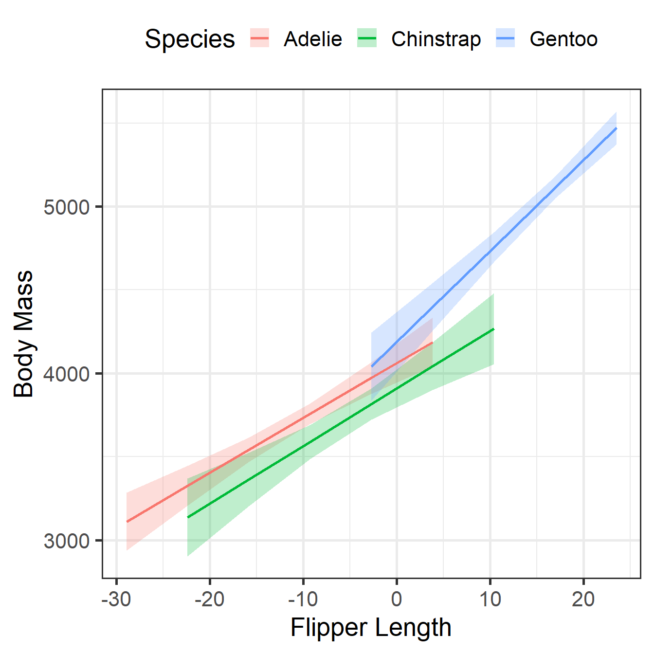

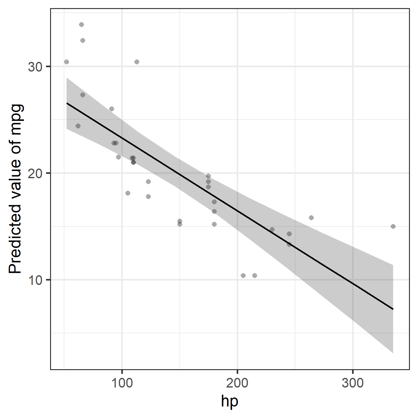
CDM Simple Slopes

estimate_slopes(
  model = cdm_fs, 
  trend = "flipper_len", 
  by = "species"
)

Estimated Marginal Effects

species   | Slope |   SE |         95% CI | t(336) |      p
-----------------------------------------------------------
Adelie    | 32.83 | 4.63 | [23.73, 41.93] |   7.10 | < .001
Chinstrap | 34.57 | 6.33 | [22.11, 47.03] |   5.46 | < .001
Gentoo    | 54.62 | 5.17 | [44.46, 64.79] |  10.57 | < .001

Marginal effects estimated for flipper_len
Type of slope was dY/dX

Notice the Gentoo slope (54.6) is the Adelie slope (32.8) plus the interaction (21.8).

A Formula Resource

Formula	Slopes Estimated
y ~ x	\(x\)
y ~ x + w	\(x\)	\(w\)
y ~ x * w	\(x\)	\(w\)		\(xw\)
y ~ x + w + z	\(x\)	\(w\)	\(z\)
y ~ x * w + z	\(x\)	\(w\)	\(z\)	\(xw\)
y ~ x * (w + z)	\(x\)	\(w\)	\(z\)	\(xw\)	\(xz\)
y ~ (x + w + z)^2	\(x\)	\(w\)	\(z\)	\(xw\)	\(xz\)	\(wz\)
y ~ x * w * z	\(x\)	\(w\)	\(z\)	\(xw\)	\(xz\)	\(wz\)	\(xwz\)

Note that predictors can be continuous or discrete, but if a discrete predictor has more than two levels, you will end up with additional slopes due to dummy coding. To represent \(g\) groups, it will create \(g-1\) dummy codes (with a slope for each).

Linearity Assumption

Overview

• The Assumption: The model matches the shape of the data
  • We assume the relationship is a straight line (additive)
  • Intuition: A one-unit increase in \(x\) always produces the same increase in \(y\)
• The Problem: Mismatched shapes (misspecification)
  • Real relationships are often curved (practice effects, diminishing returns)
  • If we force a straight line onto a curve, our predictions will be wrong
• The Solution: Flexible modeling
  • Simple Fix: For basic curves, we add polynomial (e.g., quadratic) terms
  • Advanced Fix: For complex shapes, we use generalized additive modeling (GAM)
  • Takeaway: We transform the predictors to allow the model to bend

Example

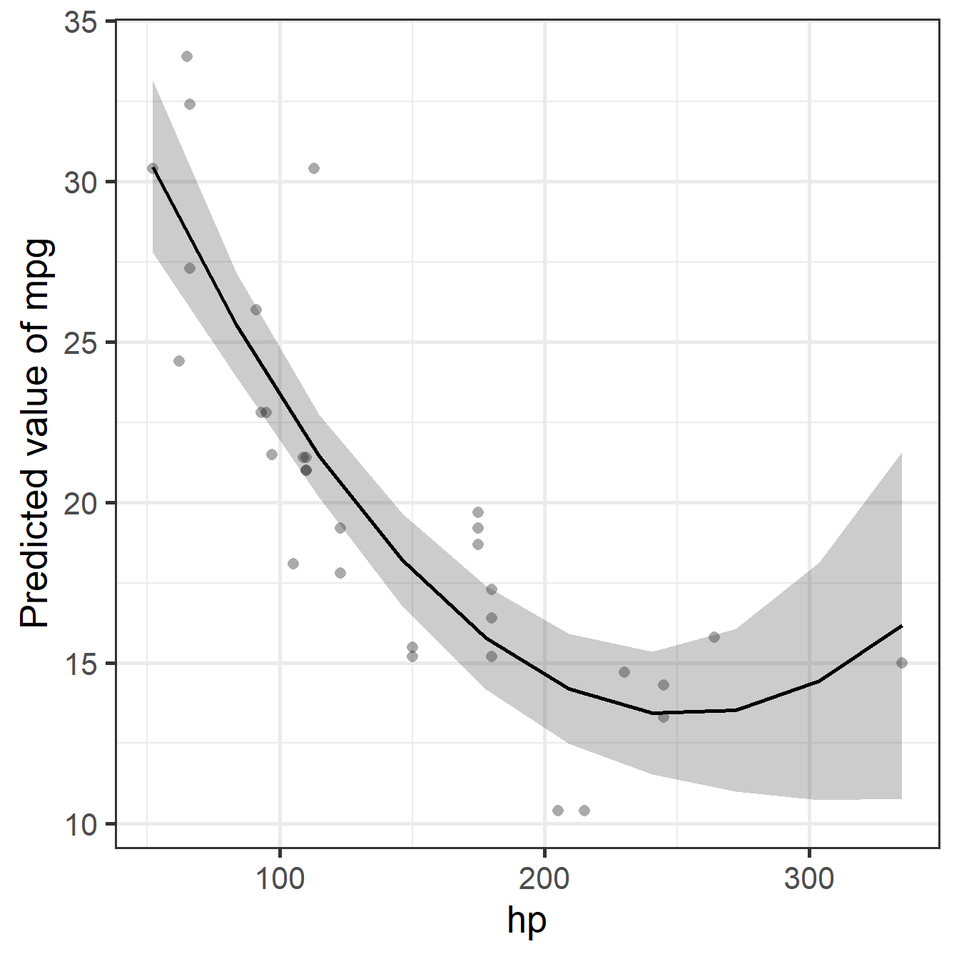
# Does horsepower predict mpg?
fit_line <- lm(
  formula = mpg ~ 1 + hp, 
  data = mtcars
)
pred_line <- estimate_relation(
  model = fit_line, 
  by = "hp"
)
plot(pred_line, show_data = TRUE)

Note: Adding horsepower hurts fuel economy, but this levels off (you can’t go below 0 mpg), creating the curve that the linear model misses.

Diagnostic

# The reference line looks bad - major violation
check_model(fit_line, check = "linearity", base_size = 16)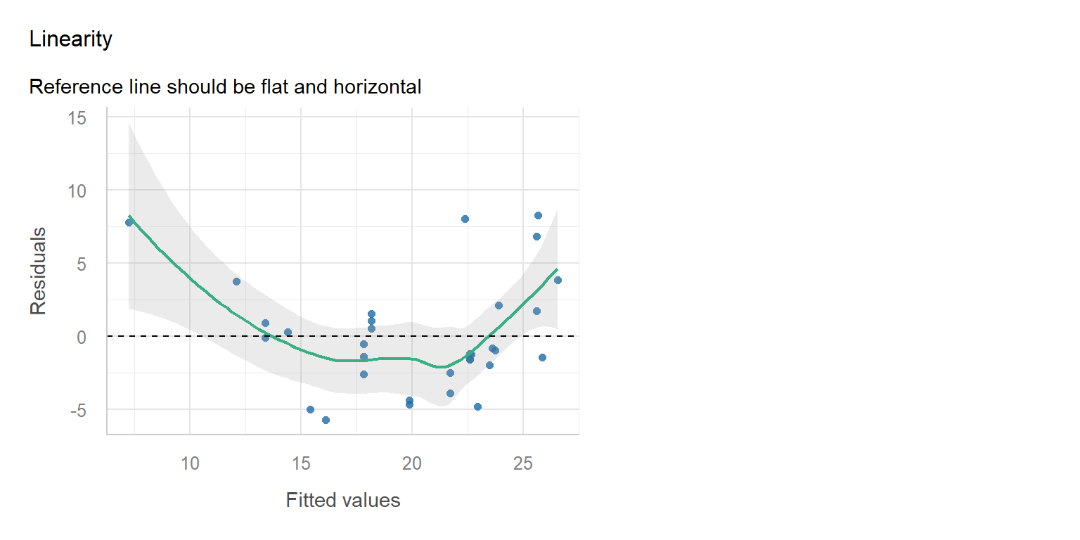

Simple Fix

• The Trick: Transform the Data, not the Parameters.
  • We can model curves by adding a squared term (\(x^2\)) as a new predictor.
  • Still Linear: \(y_i = \beta_0 + \beta_1 x_i + \beta_2 x_i^2 + \varepsilon_i\)
  • We can do this in R easily using poly(x, degree = 2) or poly(x, 2)
  • Since we are still just adding weighted terms, this remains a Linear Model (LM).
• True Non-Linear Models (The “Illegal” Move):
  • Not Linear: \(y_i = \beta_0 \cdot x_i^{\beta_1}\)
  • Here, the parameter is an exponent. This requires different math!

Implementation

fit_poly <- lm(
  formula = mpg ~ 1 + 
    poly(hp, 2, raw = TRUE), 
  data = mtcars
)

pred_poly <- estimate_relation(
  model = fit_poly, 
  by = "hp"
)
plot(pred_poly, show_data = TRUE)

Note: By allowing the line to bend or curve (quadratically), we capture the relationship accurately.

Homogeneity Assumption

Overview

• The Assumption: The model is equally reliable everywhere
  • We assume the error is constant for all participants
  • Intuition: The model should predict low scores as precisely as high scores
• The Problem: Uneven reliability (heteroskedasticity)
  • The model is precise for some people but wildly guessing for others
  • Visual: A “megaphone” shape (errors spread out as values increase)
  • Consequence: Standard errors are wrong (usually too small)
• The Solution: Handling the noise
  • Simple Fix: Apply heteroskedasticity-consistent (HC3) standard errors
  • Advanced Fix: Model the error variance explicitly using location–scale models
  • Takeaway: We stop assuming the noise is the same for everyone

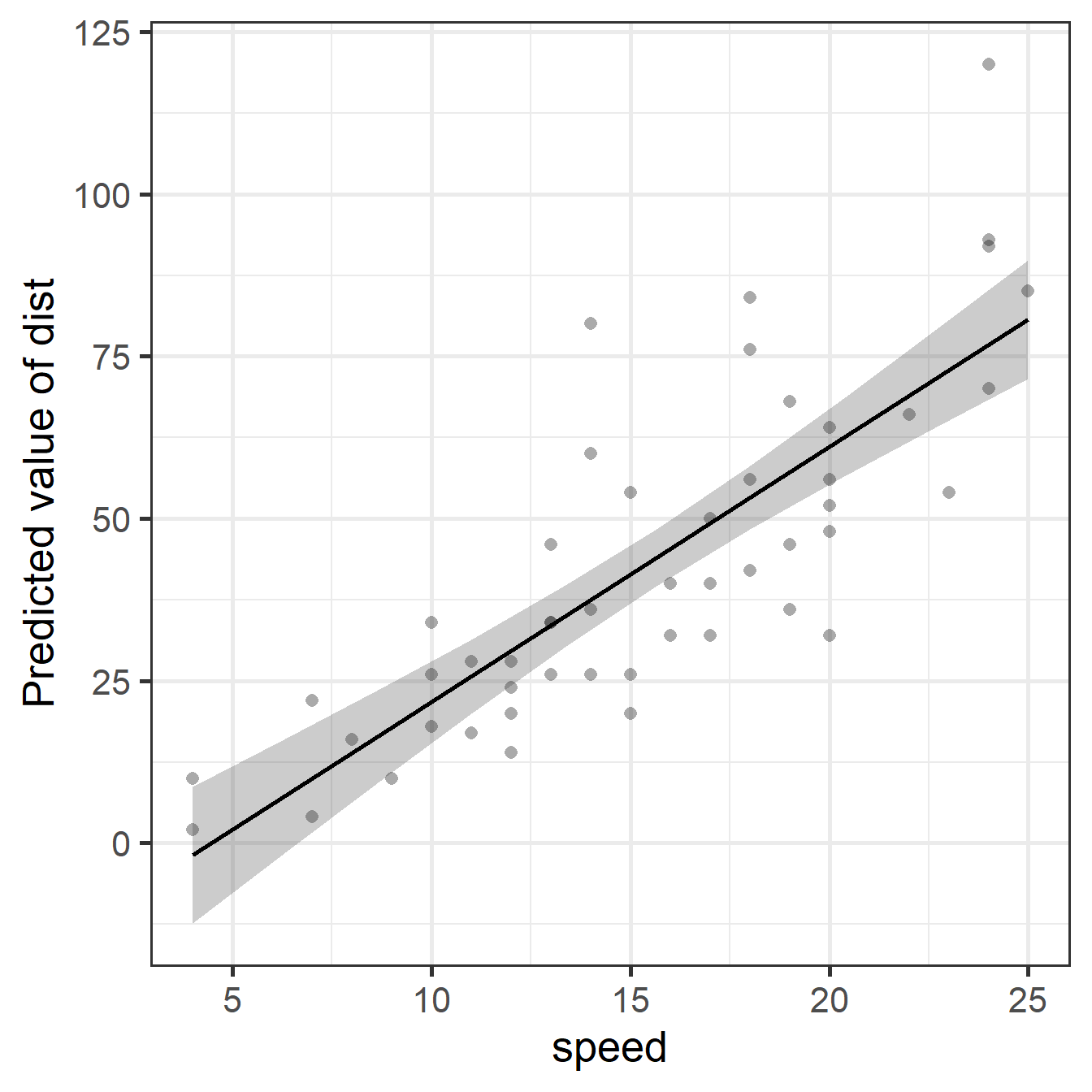
Example

# Does speed predict stop distance?
fit_cars <- lm(
  formula = dist ~ speed, 
  data = cars
)

pred_cars <- estimate_relation(
  fit_cars, 
  by = "speed"
)
plot(pred_cars, show_data = TRUE)

Note: At low speeds, points are near the line. At high speeds, they spread out. We predict distance for “slow” stops well, but not for “fast” stops.

Diagnostic

# The reference line looks fair - minor violation
check_model(fit_cars, check = "homogeneity", base_size = 16)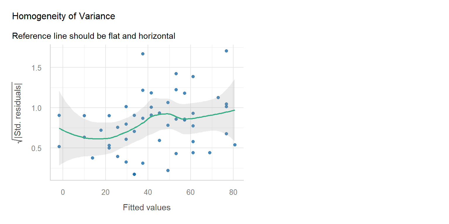

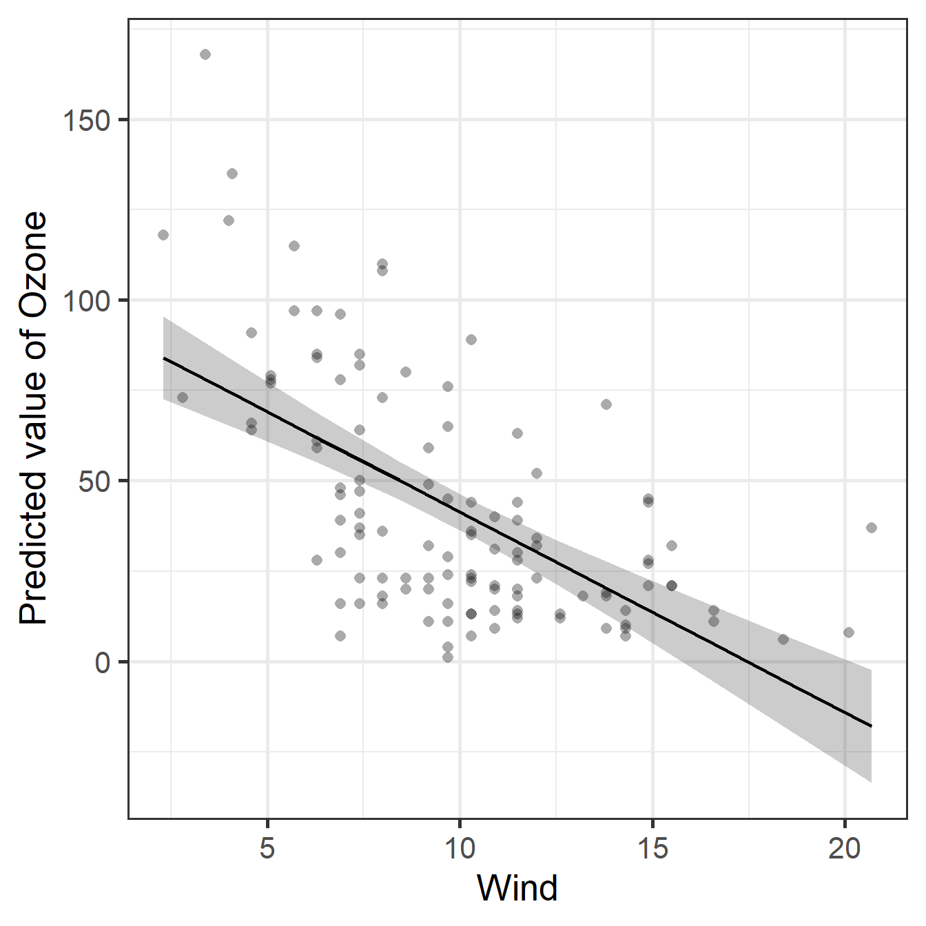
Simple Fix

• The Logic:
  • We keep the parameter point estimates unchanged
  • We penalize the Standard Errors where variance is high
  • The creates “honest” \(p\)-values that account for noise
  • We use heteroskedasticity-consistent SEs (formula HC3)
• The Intuition:
  • Standard (OLS): Assumes the “noise level” is identical for everyone. It calculates one global variance (\(\sigma^2\)) and trusts it everywhere.
  • Robust (HC3): Acknowledges that precision varies. It uses the actual squared error of each observation (\(\varepsilon_i^2\)) to estimate the variance.
  • The “Penalty”: If the model sees large errors in a specific area, it “learns” that the slope is unstable there and inflates the SE to reflect that uncertainty.

Implementation

model_parameters(fit_cars)  # standard OLS results

Parameter   | Coefficient |   SE |          95% CI | t(48) |      p
-------------------------------------------------------------------
(Intercept) |      -17.58 | 6.76 | [-31.17, -3.99] | -2.60 | 0.012 
speed       |        3.93 | 0.42 | [  3.10,  4.77] |  9.46 | < .001

model_parameters(fit_cars, vcov = "HC3") # fix

Parameter   | Coefficient |   SE |          95% CI | t(48) |      p
-------------------------------------------------------------------
(Intercept) |      -17.58 | 5.93 | [-29.51, -5.65] | -2.96 | 0.005 
speed       |        3.93 | 0.43 | [  3.07,  4.79] |  9.20 | < .001

Observation: In this case, the penalty is small! But we pay it anyway because it ensures our inferences and conclusions are valid.

Normality Assumption

Overview

• The Assumption: The errors follow a bell curve
  • We assume the residuals are normally distributed around zero
  • Intuition: Most prediction errors are small; extreme errors are rare and symmetric
• The Problem: Non-normality of error
  • The residuals might be skewed, bounded, or have “heavy tails”
  • Consequence: p-values are untrustworthy, especially in small samples (\(n<50\))
• The Solution: Changing the Assumptions
  • Simple Fix: We resample or “bootstrap” our own data to build empirical estimates of uncertainty without assuming any shape for the sampling distribution
  • Advanced Fix: We explicitly model the error distribution using Generalized Linear Modeling (GLM), e.g., logistic for binary, poisson for counts, cumulative for ordinal
  • Takeaway: We stop forcing non-normal data into a normal shape.

Example

# Does wind speed predict ozone?
fit_ozone <- lm(
  formula = Ozone ~ Wind, 
  data = airquality
)

pred_ozone <- estimate_relation(
  model = fit_ozone, 
  by = "Wind"
)
plot(pred_ozone, show_data = TRUE)

Note: The model fits a straight line, but there are outliers and negative Ozone (impossible) is being predicted.

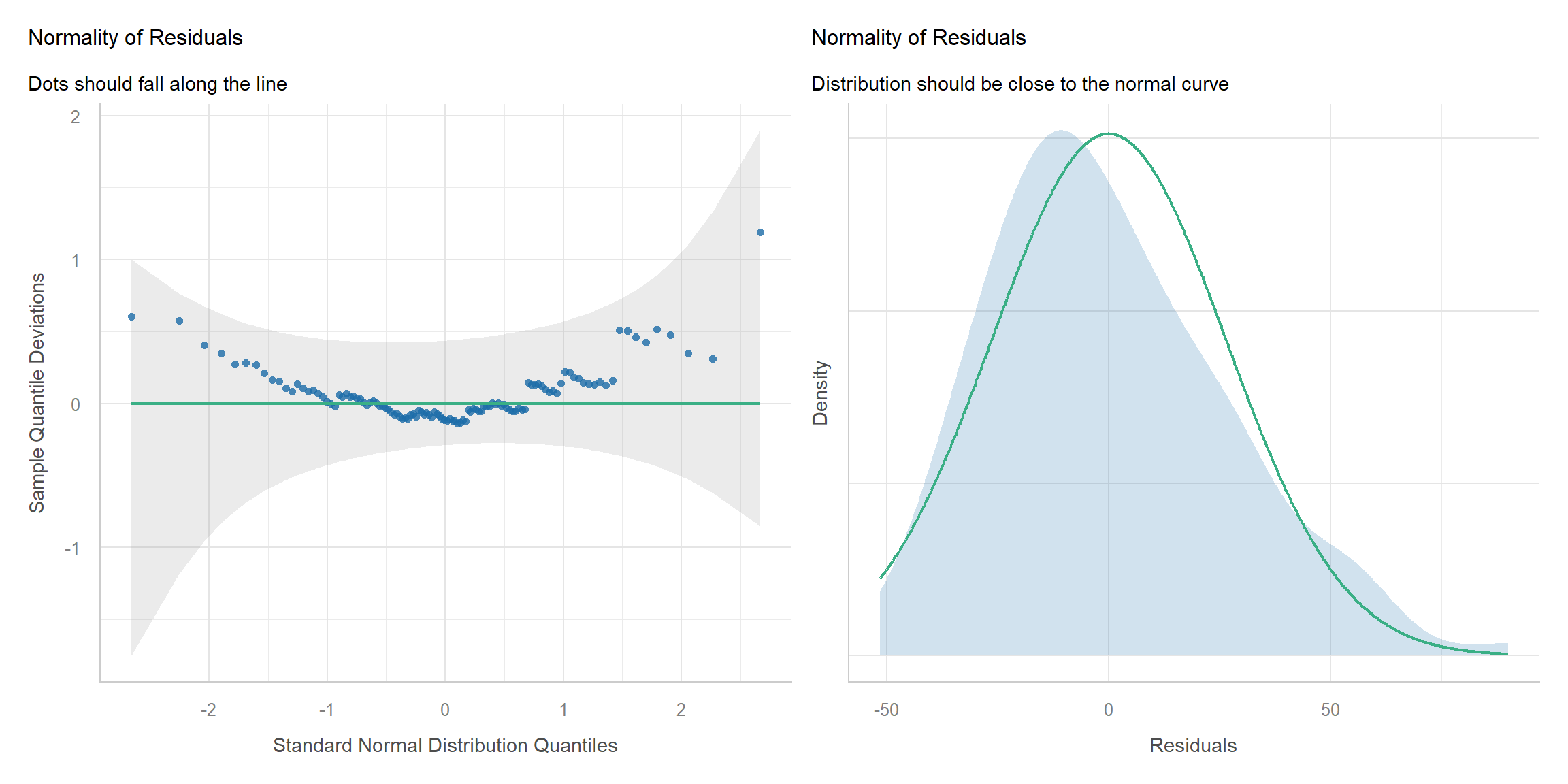
Diagnostic

# Distributions look fair - minor violation
check_model(fit_ozone, check = c("qq", "normality"), base_size = 18)

Simple Fix

• The Logic:
  • If the residuals aren’t Normal, the formulas for SEs and CIs are wrong
  • Resampling methods like bootstrapping skips the formulas
  • We simulate repeating the experiment 2,000 times using our own data
  • This is done by sampling \(n\) observations each time with replacement
  • If 95% of those simulations show a negative slope, the effect is reliable
• The Intuition:
  • Standard (Parametric): “I assume the sampling distribution is a perfect bell curve.”
  • Bootstrap (Non-Parametric): “I don’t assume anything about the shape of the sampling distribution. I built the distribution myself by reshuffling the data.”

Implementation

model_parameters(fit_ozone) # standard OLS results

Parameter   | Coefficient |   SE |          95% CI | t(114) |      p
--------------------------------------------------------------------
(Intercept) |       96.87 | 7.24 | [82.53, 111.21] |  13.38 | < .001
Wind        |       -5.55 | 0.69 | [-6.92,  -4.18] |  -8.04 | < .001

model_parameters(fit_ozone, bootstrap = TRUE, iterations = 2000) # fix

Parameter   | Coefficient |          95% CI |      p
----------------------------------------------------
(Intercept) |       97.09 | [80.15, 114.61] | < .001
Wind        |       -5.56 | [-7.15,  -4.07] | < .001

Observation: The confidence interval changed slightly. Because we had a decent sample size (\(n=153\)), the Central Limit Theorem helped the standard approach. In smaller samples, the difference would likely be larger.

Independence Assumption

Preview

• The Assumption: The residuals are independent
  • We assume that every data point provides unique, unrelated information
  • Intuition: Knowing the error for observation \(i\) tells us nothing about observation \(j\)
• The Problem: Clustering and dependency
  • Observations are often related (e.g., repeated measures, students nested in schools)
  • Consequence: The “effective” sample size is much smaller than \(n\), leading to an overestimation of confidence (e.g., \(p\)-values are too small, Type I errors)
• The Solution: Addressing the structure
  • Simple Fix: Cluster-robust SEs or Fixed effects (dummy codes) per cluster
  • Advanced Fix: Generalized estimating equations (GEE) or Multilevel models (MLM)
  • Takeaway: We stop assuming rows are independent and model the hierarchy