Multilevel Modeling

Centering and Degrouping

Spring 2026 | CLAS | PSYC 894
Jeffrey M. Girard | Lecture 08a

Roadmap

Conceptual Foundations
- Centering and Standardizing
- Manifest Decomposition
Applications and Interpretation
- Data Preparation
- Model Building

Conceptual Foundations

The Need for a Meaningful Zero

The intercept is the expected value of \(y\) when all predictors equal zero
For categorical predictors, zero is the reference group
For continuous predictors, a value of zero might be mathematically possible but practically meaningless
- What does a prediction at age 0 mean when studying adults?
- If a school cannot have 0 funding, the intercept becomes uninterpretable

The Solution: We often transform our continuous predictors so that zero represents a meaningful baseline (usually the mean)
This is particularly valuable when the intercept is of substantive interest or when the variable is involved in interactions

Centering Level 2 Predictors

Level 2 predictors represent cluster-level characteristics
We typically center these using Grand Mean Centering (GMC)
- We subtract the overall (grand) mean from each cluster’s score
- \(z_j^{(c)} = z_j - \bar{z}\)

Interpretation after GMC:
- A value of 0 now represents the average cluster in the sample
- Positive values are above and negative values are below average
- The intercept becomes the expected outcome for an average cluster

Standardizing Level 2 Predictors

Sometimes we want our predictors to be on a standardized scale
For Level 2 variables, this process is (or should be) straightforward
- We subtract the grand mean and divide by the grand standard deviation
- \(z_j^{(s)} = \frac{z_j - \bar{z}}{SD(z)}\)

Interpretation after Standardizing:
- A value of 0 still represents the average cluster
- A value of 1 represents a cluster that is 1 SD above the mean
- The slope tells us the expected change in \(y\) for a 1-SD increase in \(z\)

The Problem with Level 1 Predictors

Level 1 predictors like student socioeconomic status (SES) are trickier
A student’s raw SES score actually contains two different pieces of information rolled into one:
1. Within-Cluster Variance: How wealthy is this student compared to their classmates? (The “Frog Pond” effect)
2. Between-Cluster Variance: How wealthy is the school this student attends? (The Compositional effect)

If we just enter raw L1 SES into the model, the software estimates a single slope that aggressively blends these two effects together
This is called a conflated effect and it can severely bias our results

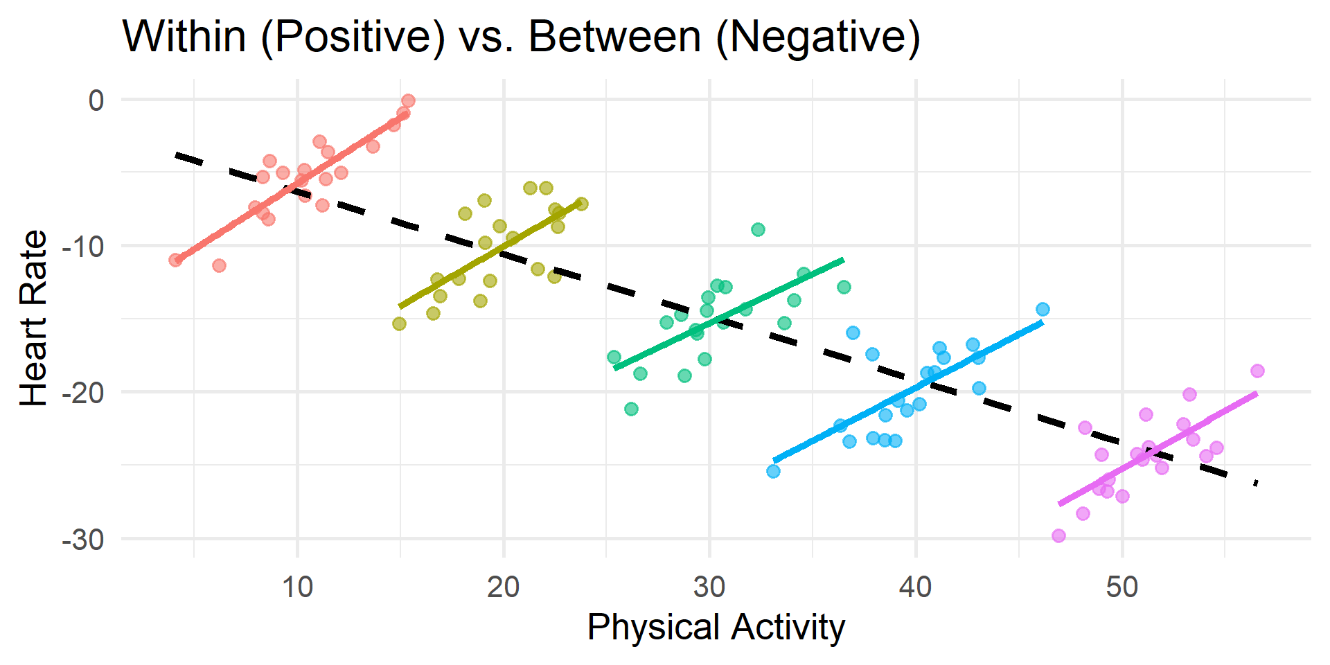
Multilevel Fallacies and Paradoxes

If we ignore this and report the conflated effect anyway, we risk falling into:

The Ecological Fallacy: Assuming that relationships observed at the group level (L2) automatically apply to individuals (L1)
The Atomistic Fallacy: Assuming that relationships observed at the individual level (L1) automatically apply to groups (L2)
Simpson’s Paradox: The relationship at the aggregate level (L2) is entirely different compared to the relationship at the individual level (L1)

“If the model does not properly account for the fact that there are different relationships between the predictor and the outcome at different levels, we end up with a slope that is an uninterpretable blend of the within-person and between-person slopes.” — Hamaker & Muthén (2020)

Visualizing Simpson’s Paradox

Manifest Decomposition (Degrouping)

To fix this, we “degroup” the L1 predictor into two new variables

The Between-Cluster Component (L2)
- We calculate the mean of the L1 variable for each cluster
- \(x_j^{(b)}\) represents the school’s raw average SES
The Within-Cluster Component (L1)
- We subtract the cluster mean from the student’s raw score
- This specific math is called Cluster Mean Centering (CMC)
- \(x_{ij}^{(wc)} = x_{ij} - x_j^{(b)}\)
- This represents the student’s relative standing within their school

The Magic of Orthogonality

There is a hidden mathematical benefit to Manifest Decomposition
Because we calculate \(x_{ij}^{(wc)}\) by subtracting the cluster mean, the sum of these within-cluster scores is exactly 0 for every school

What this means mathematically:
- The between-cluster component \(x_j^{(b)}\) and the within-cluster component \(x_{ij}^{(wc)}\) are orthogonal, i.e., completely uncorrelated (\(r = 0\))

Why this matters practically:
- In regression, correlated predictors compete for explained variance
- Because our components are orthogonal, they do not compete

Do We Always Need Both Components?

What if you only care about the within-cluster effect? Can you just use cluster mean centering (CMC) and ignore the cluster means?

Statistically: Yes. Using only the CMC variable will give you an unbiased estimate of the purely within-cluster slope

Practically: Leaving the cluster means out is usually a missed opportunity!
- Including the between-cluster component \(x_j^{(b)}\) helps explain Level 2 variance and improve the model
- It allows you to estimate the between-cluster effect. This tells you if attending a wealthy school provides a unique benefit above and beyond a student’s individual wealth

Standardizing Level 1 Predictors

What if we want to standardize a Level 1 predictor?
We must be careful not to re-conflate the variance we just separated
The Rule: Standardize Level 1 variables only after degrouping them

The between-cluster component \(x_j^{(bs)}\) is standardized using the mean and SD of the unique cluster means
The within-cluster component \(x_{ij}^{(ws)}\) is standardized using a mean of 0 and the pooled within-cluster SD
This ensures a 1-unit change accurately represents a 1-SD shift at the correct level of analysis

What About Standardizing Y?

In standard regression (OLS), we often standardize both predictors and the outcome to get fully standardized coefficients
In multilevel modeling, we typically only standardize the predictors and leave the outcome (\(y\)) in its raw metric

Why do we leave Y raw?

The variability of \(y\) is partitioned across multiple levels (e.g., within-cluster \(\sigma\) and between-cluster \(\tau_{00}\))
Standardizing \(y\) globally distorts this variance partitioning and makes the random effects very difficult to interpret
By only standardizing our predictors, we get “partially standardized” slopes: A 1-SD increase in the predictor leads to a \(\gamma\) unit change in the raw outcome

Best Practice Recommendations

Here is a summary checklist for continuous variables in multilevel models.

The Outcome Variable: Leave the outcome \((y)\) in its raw, uncentered metric so variance components remain interpretable
Meaningful Intercepts: Transform continuous predictors when 0 is not naturally meaningful or when the variable is involved in interactions
Level 2 Predictors: Grand mean center or standardize directly
Level 1 Predictors: Degroup into between-cluster and within-cluster components
Standardizing L1: Degroup first, then standardize the resulting components independently
Random Slopes: If you are testing cross-level or compositional interactions, the Level 1 component must have a random slope

Data Preparation

The Weighting Problem

When we work with Level 1 data (one row per student), Level 2 variables (like school funding or proportion going to university) are repeated for every student in that school

If we simply run center(puniv) on this dataset, the software calculates the mean across all rows, not all schools

Why is this a problem?

It weights the grand mean and standard deviation by cluster size
A school with 1,000 students pulls the mean 10 times harder than a school with 100 students!
The resulting variables are biased toward larger clusters and no longer represent the typical school

The “Split, Transform, Join” Workflow

To safely center and standardize our variables without size bias, we need to explicitly separate our data by level

Split: Create a dataset with exactly one row per cluster (Level 2)
Transform (L2): Safely apply Grand Mean Centering and Standardizing to this unweighted data
Join: Merge these perfect Level 2 variables back into the Level 1 variables
Transform (L1): Safely apply Cluster Mean Centering and Standardizing to the Level 1 variables

Step 1: Prep the Level 2 Data

First, we load our data and create a Level 2 dataset. We grab our L2 predictor (puniv) and calculate the raw cluster mean for our L1 predictor (ses_b)

library(tidyverse)

dat_raw <- read_csv("heck2011.csv") |>
  mutate(school = factor(school))

dat_l2 <- dat_raw |>
  summarize(
    .by = school,
    puniv = first(puniv), 
    ses_b = mean(ses, na.rm = TRUE)
  )

Because this dataset has exactly one row per school, we can safely center and standardize without weighting biases!

Step 1: Transform the Level 2 Data

dat_l2 <- dat_l2 |>
  # Apply Grand Mean Centering and Standardizing to L2
  mutate(
    puniv_c = center(puniv),
    ses_bc  = center(ses_b),
    puniv_s = standardize(puniv),
    ses_bs  = standardize(ses_b)
  )
glimpse(dat_l2)

Rows: 419
Columns: 7
$ school  <fct> 1, 2, 3, 4, 5, 6, 7, 8, 9, 10, 11, 12, 13, 14, 15, 16, 17, 18,…
$ puniv   <dbl> 0.08333333, 1.00000000, 0.33333333, 1.00000000, 1.00000000, 1.…
$ ses_b   <dbl> -0.2667500, 0.6799231, -0.5480000, 0.8159412, -0.3892941, 0.25…
$ puniv_c <dw_trnsf> -0.7816475, 0.1350191, -0.5316475, 0.1350191, 0.1350191, …
$ ses_bc  <dw_trnsf> -0.2862979, 0.6603752, -0.5675479, 0.7963933, -0.4088420,…
$ puniv_s <dw_trnsf> -2.8454676, 0.4915165, -1.9353811, 0.4915165, 0.4915165, …
$ ses_bs  <dw_trnsf> -0.5883235, 1.3570281, -1.1662739, 1.6365364, -0.8401436,…

Step 2: Prep the Level 1 Data

Next, take the original L1 data and join our new L2 data into it

dat <- dat_raw |>
  # Drop the raw L2 variable to avoid duplicates during the join
  select(-puniv) |> 
  left_join(dat_l2, by = "school")

Finally, we calculate the within-cluster component. Because cluster-mean-centered scores always sum to zero within a cluster, standardize() automatically calculates the correct pooled within-cluster standard deviation.

Step 2: Transform the Level 1 Data

dat <- dat |>
  mutate(
    ses_wc = ses - ses_b, 
    ses_ws = standardize(ses_wc) 
  )
dat |> select(school, ses_b, ses, ses_wc, ses_ws) |> glimpse()

Rows: 6,871
Columns: 5
$ school <fct> 1, 1, 1, 1, 1, 1, 1, 1, 1, 1, 1, 1, 2, 2, 2, 2, 2, 2, 2, 2, 2, …
$ ses_b  <dbl> -0.2667500, -0.2667500, -0.2667500, -0.2667500, -0.2667500, -0.…
$ ses    <dbl> 0.586, 0.304, -0.544, -0.848, 0.001, -0.106, -0.330, -0.891, 0.…
$ ses_wc <dbl> 0.852750000, 0.570750000, -0.277250000, -0.581250000, 0.2677500…
$ ses_ws <dw_trnsf> 1.409368976, 0.943297969, -0.458220520, -0.960651677, 0.44…

Model Building

Model 1: Establishing Main Effects

Let’s predict math scores using student wealth and school wealth

The Predictors:
- ses_wc: The student’s relative wealth compared to their peers
- ses_bc: The school’s overall average wealth
- puniv_c: The school’s university attendance rate (as an L2 covariate)

The Goal:
- By including both SES components, we avoid the conflated effect problem and can tease apart the unique effects of both components
- We will also compare the use of centered and standardized predictors

Model 1C: Path Diagram

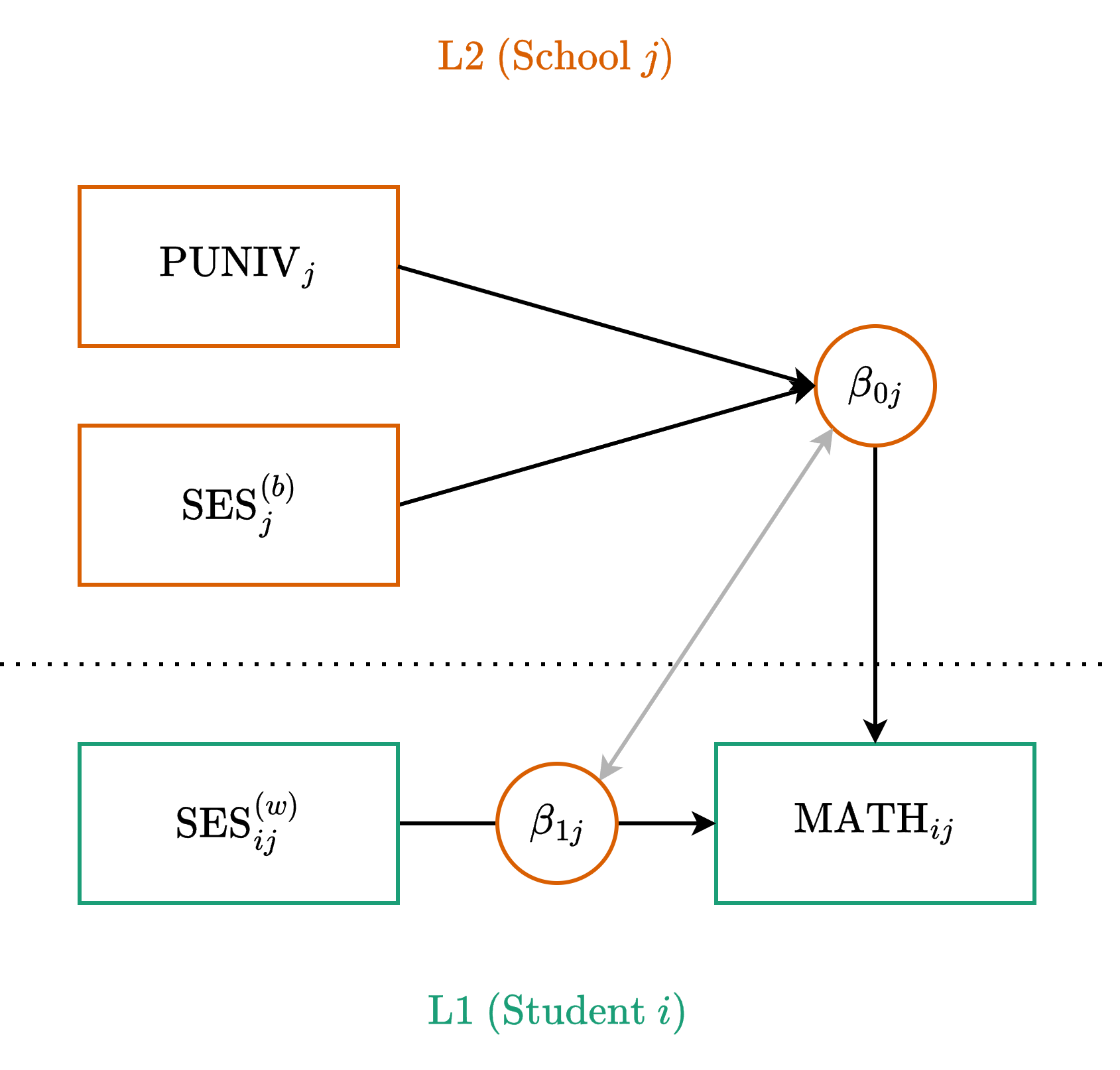
Model 1C: Centered Equations

Level One (Observation)

\[ y_{ij} = \beta_{0j} + \beta_{1j} x_{ij}^{(wc)} + \color{#4daf4a}{e_{ij}} \]

Level Two (Cluster)

\[ \begin{align} \beta_{0j} &= \color{#377eb8}{\gamma_{00}} + \color{#377eb8}{\gamma_{01}} x_j^{(bc)} + \color{#377eb8}{\gamma_{02}} z_j^{(c)} + \color{#e41a1c}{u_{0j}} \\ \beta_{1j} &= \color{#377eb8}{\gamma_{10}} + \color{#e41a1c}{u_{1j}} \end{align} \]

\(\gamma_{10}\) is the fixed within-cluster effect
\(\gamma_{01}\) is the fixed between-cluster effect
\(\gamma_{02}\) is the fixed effect of our L2 covariate

Model 1C: Mixed Equation

Substitute the L2 equations directly into the L1 equation:

\[ y_{ij} = \underbrace{\color{#377eb8}{\gamma_{00}} + \color{#377eb8}{\gamma_{01}} x_j^{(bc)} + \color{#377eb8}{\gamma_{02}} z_j^{(c)} + \color{#377eb8}{\gamma_{10}} x_{ij}^{(wc)}}_{\text{Fixed}} + \underbrace{\color{#e41a1c}{u_{0j}} + \color{#e41a1c}{u_{1j}} x_{ij}^{(wc)}}_{\text{Random}} + \color{#4daf4a}{e_{ij}} \]

Formula Syntax

y ~ 1 + x_between + x_within + z_l2 + (1 + x_within | cluster)

Our Example

math ~ 1 + ses_bc + ses_wc + puniv_c + (1 + ses_wc | school)

Model 1C: Fitting the Model

fit1c <- lmer(
  math ~ 1 + ses_bc + ses_wc + puniv_c + (1 + ses_wc | school), 
  data = dat
)
model_parameters(fit1c, effects = "fixed")

# Fixed Effects

Parameter   | Coefficient |   SE |         95% CI | t(6863) |      p
--------------------------------------------------------------------
(Intercept) |       57.66 | 0.12 | [57.42, 57.90] |  470.53 | < .001
ses bc      |        5.60 | 0.26 | [ 5.09,  6.11] |   21.54 | < .001
ses wc      |        3.19 | 0.17 | [ 2.86,  3.51] |   19.14 | < .001
puniv c     |        1.52 | 0.47 | [ 0.60,  2.43] |    3.25 | 0.001

Model 1C: Interpretation

Because our predictors are centered, the coefficients represent changes in raw math points for a 1-unit increase in the raw predictor

Intercept (57.66): The expected math score for an average student (ses_wc = 0) at an average school (ses_bc = 0 and puniv_c = 0)
ses_bc (5.60): Controlling for student wealth and university attendance, a 1-unit increase in a school’s overall SES is associated with a 5.60 point increase in math
ses_wc (3.19): Controlling for school factors, a 1-unit increase in a student’s relative wealth is associated with a 3.19 point increase in math
puniv_c (1.52): Controlling for school and student SES, a 1-unit increase in the university attendance rate (e.g., from 10% to 11%) is associated with a 1.52 point increase in math

Model 1S: Standardized Equations

The structure remains identical, but we swap in the standardized components

Level One (Observation)

\[ y_{ij} = \beta_{0j} + \beta_{1j} x_{ij}^{(ws)} + \color{#4daf4a}{e_{ij}} \]

Level Two (Cluster)

\[ \begin{align} \beta_{0j} &= \color{#377eb8}{\gamma_{00}} + \color{#377eb8}{\gamma_{01}} x_j^{(bs)} + \color{#377eb8}{\gamma_{02}} z_j^{(s)} + \color{#e41a1c}{u_{0j}} \\ \beta_{1j} &= \color{#377eb8}{\gamma_{10}} + \color{#e41a1c}{u_{1j}} \end{align} \]

Because our inputs are standardized, the resulting gammas will tell us the expected change in math points for a 1-SD increase in the predictors.

Model 1S: The Standardized Model

fit1s <- lmer(
  math ~ 1 + ses_bs + ses_ws + puniv_s + (1 + ses_ws | school), 
  data = dat
)
model_parameters(fit1s, effects = "fixed")

# Fixed Effects

Parameter   | Coefficient |   SE |         95% CI | t(6863) |      p
--------------------------------------------------------------------
(Intercept) |       57.66 | 0.12 | [57.42, 57.90] |  470.52 | < .001
ses bs      |        2.73 | 0.13 | [ 2.48,  2.98] |   21.54 | < .001
ses ws      |        1.93 | 0.10 | [ 1.73,  2.12] |   19.14 | < .001
puniv s     |        0.42 | 0.13 | [ 0.17,  0.67] |    3.25 | 0.001

Model 1S: Interpretation

Because our predictors are standardized and our outcome is raw, the coefficients represent changes in raw math points for a 1-SD increase.

Intercept (57.66): The expected math score for an average student (ses_ws = 0) at an average school (ses_bs = 0 and puniv_s = 0)
ses_bs (2.73): Controlling for student wealth and university attendance, a 1-SD increase in a school’s overall SES is associated with a 2.73 point increase in math
ses_ws (1.93): Controlling for school factors, a 1-SD increase in a student’s relative wealth is associated with a 1.93 point increase in math
puniv_s (0.42): Controlling for school and student SES, a 1-SD increase in university attendance rate is associated with a 0.42 point increase in math

Model 2: Moving to Moderation

In Model 1, we established the main effects. We know that being relatively wealthy is beneficial (the within-cluster effect) and attending a wealthy school is beneficial (the between-cluster effect)

A New Question: Does the benefit of relative wealth depend on the overall wealth of the school?
- In other words, does being the richest kid in school matter more if you are at a poor school versus a wealthy school?

To test this, we can allow the school’s average SES to moderate the slope of the student’s relative SES (for simplicity, we will also drop puniv here)
Because both the predictor and the moderator originate from the same variable, this is often called a compositional interaction or self-moderation

Model 2C: Path Diagram

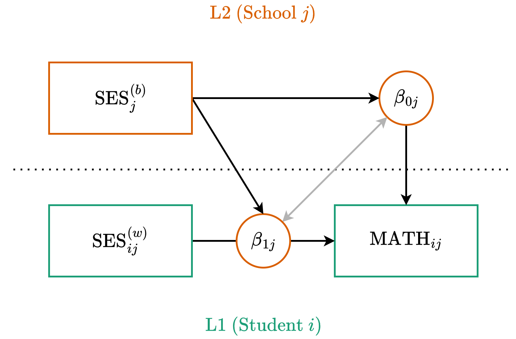
Model 2C: Centered Equations

Level One (Observation)

\[ y_{ij} = \beta_{0j} + \beta_{1j} x_{ij}^{(wc)} + \color{#4daf4a}{e_{ij}} \]

Level Two (Cluster)

\[ \begin{align} \beta_{0j} &= \color{#377eb8}{\gamma_{00}} + \color{#377eb8}{\gamma_{01}} x_j^{(bc)} + \color{#e41a1c}{u_{0j}} \\ \beta_{1j} &= \color{#377eb8}{\gamma_{10}} + \underbrace{\color{#377eb8}{\gamma_{11}} x_j^{(bc)}}_{\text{New}} + \color{#e41a1c}{u_{1j}} \end{align} \]

Model 2C: Mixed Equation

Substitute the L2 equations directly into the L1 equation:

\[ y_{ij} = \underbrace{\color{#377eb8}{\gamma_{00}} + \color{#377eb8}{\gamma_{01}} x_j^{(bc)} + \color{#377eb8}{\gamma_{10}} x_{ij}^{(wc)} + \color{#377eb8}{\gamma_{11}} x_j^{(bc)} x_{ij}^{(wc)}}_{\text{Fixed}} + \dots \] \[ \dots + \underbrace{\color{#e41a1c}{u_{0j}} + \color{#e41a1c}{u_{1j}} x_{ij}^{(wc)}}_{\text{Random}} + \color{#4daf4a}{e_{ij}} \]

Formula Syntax

y ~ 1 + x_between * x_within + (1 + x_within | cluster)

Our Example

math ~ 1 + ses_bc * ses_wc + (1 + ses_wc | school)

Model 2C: Centered Interaction

fit2c <- lmer(
  math ~ 1 + ses_bc * ses_wc + (1 + ses_wc | school), 
  data = dat
)
model_parameters(fit2c, effects = "fixed")

# Fixed Effects

Parameter       | Coefficient |   SE |         95% CI | t(6863) |      p
------------------------------------------------------------------------
(Intercept)     |       57.67 | 0.12 | [57.42, 57.91] |  465.72 | < .001
ses bc          |        5.88 | 0.25 | [ 5.39,  6.38] |   23.25 | < .001
ses wc          |        3.17 | 0.17 | [ 2.84,  3.50] |   18.84 | < .001
ses bc × ses wc |       -0.29 | 0.37 | [-1.02,  0.45] |   -0.77 | 0.444

Model 2C: Interpretation

Intercept (57.67): The expected math score for an average-SES student (ses_wc = 0) at an average-SES school (ses_bc = 0)
ses_bc (5.88): For a student with average relative wealth, a 1-unit increase in their school’s average SES is associated with a 5.88 point increase in math
ses_wc (3.17): At an average-SES school, a 1-unit increase in a student’s relative wealth is associated with a 3.17 point increase in math
ses_bc \(\times\) ses_wc (–0.29): The interaction is near zero and non-significant. The benefit of being relatively wealthy compared to your peers operates similarly regardless of whether you attend a poor school or a wealthy school

Model 2C: Visualizing the Interaction

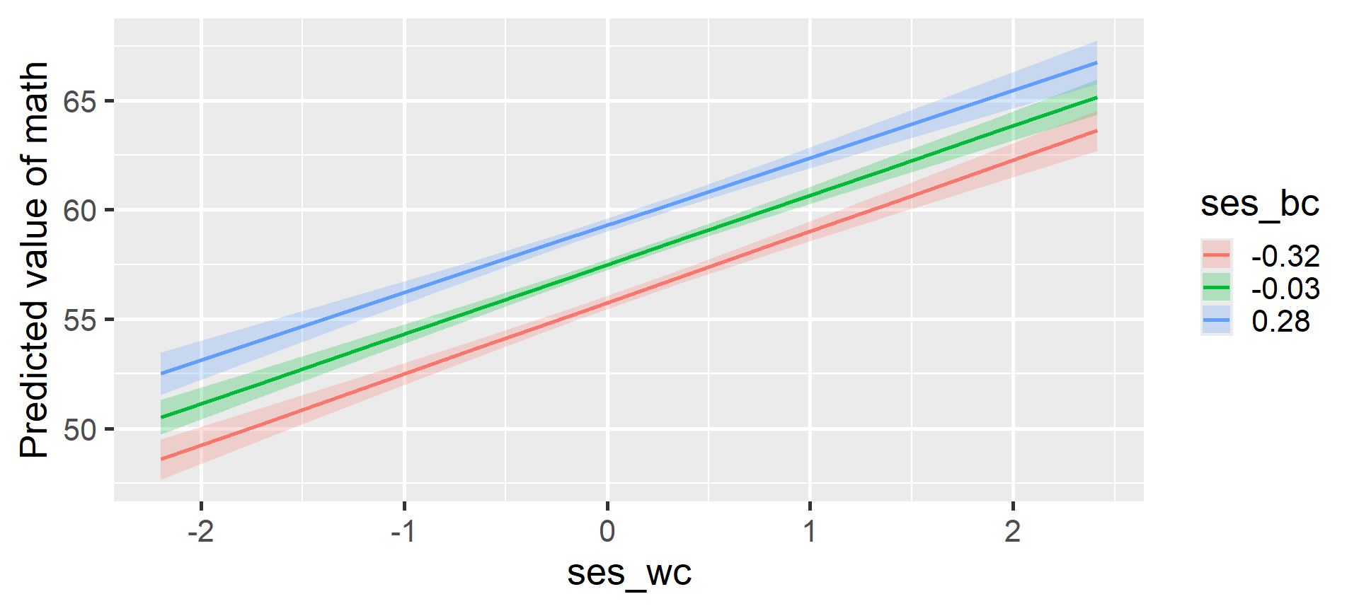
plot(estimate_relation(fit2c, by = c("ses_wc", "ses_bc=[quartiles]")))

Model 2C: Simple Slopes Analysis

estimate_slopes(fit2c, trend = "ses_wc", by = "ses_bc=[quartiles]")

Estimated Marginal Effects

ses_bc | Slope |   SE |       95% CI | t(6863) |      p
-------------------------------------------------------
-0.32  |  3.26 | 0.19 | [2.88, 3.64] |   16.82 | < .001
-0.03  |  3.18 | 0.17 | [2.85, 3.51] |   19.00 | < .001
0.28   |  3.09 | 0.21 | [2.68, 3.50] |   14.81 | < .001

Marginal effects estimated for ses_wc
Type of slope was dY/dX

The positive effect of relative SES remains stable and significant across schools with low, medium, and high average SES

Model 2S: Standardized Equations

Finally, we compare with standardized (s) predictors

Level One (Observation)

\[ y_{ij} = \beta_{0j} + \beta_{1j} x_{ij}^{(ws)} + \color{#4daf4a}{e_{ij}} \]

Level Two (Cluster)

\[ \begin{align} \beta_{0j} &= \color{#377eb8}{\gamma_{00}} + \color{#377eb8}{\gamma_{01}} x_j^{(bs)} + \color{#e41a1c}{u_{0j}} \\ \beta_{1j} &= \color{#377eb8}{\gamma_{10}} + \color{#377eb8}{\gamma_{11}} x_j^{(bs)} + \color{#e41a1c}{u_{1j}} \end{align} \]

Model 2S: Standardized Interaction

fit2s <- lmer(
  math ~ 1 + ses_bs * ses_ws + (1 + ses_ws | school), 
  data = dat
)
model_parameters(fit2s, effects = "fixed")

# Fixed Effects

Parameter       | Coefficient |   SE |         95% CI | t(6863) |      p
------------------------------------------------------------------------
(Intercept)     |       57.67 | 0.12 | [57.42, 57.91] |  465.72 | < .001
ses bs          |        2.86 | 0.12 | [ 2.62,  3.10] |   23.25 | < .001
ses ws          |        1.92 | 0.10 | [ 1.72,  2.12] |   18.84 | < .001
ses bs × ses ws |       -0.08 | 0.11 | [-0.30,  0.13] |   -0.77 | 0.444

Model 2S: Interpretation

Because our predictors are standardized and our outcome is raw, the coefficients represent changes in raw math points for a 1-SD increase

Intercept (57.67): The expected math score for an average student (ses_ws = 0) at an average school (ses_bs = 0)
ses_bs (2.86): For a student with average relative wealth, a 1-SD increase in their school’s average SES is associated with a 2.86 point increase in math
ses_ws (1.92): At an average-SES school, a 1-SD increase in a student’s relative wealth is associated with a 1.92 point increase in math
ses_bs \(\times\) ses_ws (–0.08): For every 1-SD increase in a school’s average SES, the standardized slope of relative SES changes by -0.08. This is non-significant, meaning the lines are practically parallel