Multilevel Modeling

Model Diagnostics

Spring 2026 | CLAS | PSYC 894
Jeffrey M. Girard | Lecture 13b

Roadmap

A Systematic Workflow
- Predictive Performance
- Visual Diagnostics
Sensitivity & Easy Fixes
- Bootstrapping & LSM
- DHARMa & Outliers

Part 1:
The Philosophy

Why Diagnostics?

MLMs are complex. We aren’t just estimating a line; we are estimating a system of variances.
Our standard errors and \(p\)-values assume this system is perfectly Specified, Normal, and Constant.
Small violations often don’t matter, but…
systemic violations invalidate your results.

Pass/Fail vs. Sensitivity

It is rare to see “perfect” diagnostic plots in real research.
Instead of asking “Did I pass?”, ask:
“How robust are my conclusions?”
If your finding disappears as soon as you account for a violation, the finding was likely an artifact of a bad model.

The Mathematical Foundation

Recall the equations we use to define the random components of our models. They list many of our assumptions.

Level One (Observation)

\[ \color{#4daf4a}{e_{ij}} \sim \text{Normal}(0, \color{#4daf4a}{\sigma}) \]

Level Two (Cluster)

\[ \begin{bmatrix}\color{#e41a1c}{u_{0j}}\\ \color{#e41a1c}{u_{1j}}\end{bmatrix} \sim \text{MVN}\left(\begin{bmatrix}0\\0\end{bmatrix}, \begin{bmatrix}\color{#e41a1c}{\tau_{00}} & \\ \color{#e41a1c}{\tau_{10}} & \color{#e41a1c}{\tau_{11}}\end{bmatrix}\right) \]

Assumption 1: Specification

All relevant predictors are included at the correct levels.
The random effect structure (\(\color{#e41a1c}{u_j}\)) matches the data design.
The Random Slope Rule:
If an effect varies across clusters, omitting the random slope forces that variation into the observation error (\(\color{#4daf4a}{e_{ij}}\)), which violates the independence of errors.

Assumption 2: Normality

The equations explicitly declare the distribution shape:

\(\color{#4daf4a}{e_{ij}} \sim \textbf{Normal}(0, \color{#4daf4a}{\sigma}) \therefore\text{Univariate Normal}\)
\(\color{#e41a1c}{u_{j}} \sim \textbf{MVN}(0, \color{#e41a1c}{\Sigma}) \therefore\text{Multivariate Normal}\)

We assume Level 1 errors and Level 2 deviations follow a normal curve. If the real errors are non-normal, the likelihood math “breaks” and gives biased confidence intervals.

Assumption 3: Homoscedasticity

Homoscedasticity means “constant variance.”

\[ \color{#4daf4a}{e_{ij}} \sim \text{Normal}(0, \color{#4daf4a}{\sigma}) \qquad \begin{bmatrix}\color{#e41a1c}{u_{0j}}\\ \color{#e41a1c}{u_{1j}}\end{bmatrix} \sim \text{MVN}\left(\begin{bmatrix}0\\0\end{bmatrix}, \begin{bmatrix}\color{#e41a1c}{\tau_{00}} & \\ \color{#e41a1c}{\tau_{10}} & \color{#e41a1c}{\tau_{11}}\end{bmatrix}\right) \]

The model specifies exactly one \(\color{#4daf4a}{\sigma}\) for all \(i\) and \(j\). It assumes the spread (SD) of errors is identical for every observation.
The model specifies exactly one \(\color{#e41a1c}{\tau_{00}}\) and \(\color{#e41a1c}{\tau_{11}}\). We assume cluster-level variance is constant across all clusters.

Assumption 4: Independence

We assume errors are uncorrelated with each other:

\(\color{#4daf4a}{e_{ij}}\) residuals are independent of other observations.
\(\color{#e41a1c}{u_j}\) deviations are independent across clusters
(e.g., School A’s intercept doesn’t inform School B’s).
\(\color{#4daf4a}{e_{ij}}\) and \(\color{#e41a1c}{u_j}\) are independent of each other.

Assumption 4: The Exception

Are we allowed to have any correlations?

\[ \color{#e41a1c}{\Sigma} = \begin{bmatrix}\color{#e41a1c}{\tau_{00}} & \\ \color{#e41a1c}{\tau_{10}} & \color{#e41a1c}{\tau_{11}}\end{bmatrix} \]

Yes! We explicitly model the correlation between a cluster’s intercept and its slope via \(\color{#e41a1c}{\tau_{10}}\). This “within-cluster” dependency is expected and accounted for by the model.

Part 2:
Workflow & Data

Prepping the Data

library(tidyverse)
library(glmmTMB)
library(easystats)

dat <- read_csv("diag_sim.csv") |> mutate(school = factor(school))
glimpse(dat)

Rows: 1,200
Columns: 13
$ school        <fct> 1, 1, 1, 1, 1, 1, 1, 1, 1, 1, 1, 1, 1, 1, 1, 1, 1, …
$ homework      <dbl> 9.1480604, 9.3707541, 2.8613953, 8.3044763, 6.41745…
$ iq            <dbl> 96.27276, 106.33481, 114.81480, 112.53352, 90.09217…
$ parent_ed     <dbl> 9.557333, 11.094028, 10.595360, 10.651239, 7.393954…
$ study_time    <dbl> 8.8737958, 9.0536683, 2.6985937, 7.8450080, 6.86375…
$ u0            <dbl> -4.27901645, -4.27901645, -4.27901645, -4.27901645,…
$ e_normal      <dbl> 7.06285578, 6.40985063, -2.25772138, -3.75880719, -…
$ e_het         <dbl> 24.2418425, 5.3332067, -0.3621076, 1.1654239, 4.475…
$ e_skew        <dbl> 10.0483377, -1.0081537, -1.3384338, -0.8878903, 5.9…
$ score_ideal   <dbl> 68.38879, 69.00922, 53.37842, 58.18090, 55.55666, 6…
$ score_het     <dbl> 75.94050, 57.29910, 43.79255, 51.85178, 52.89746, 4…
$ score_skew    <dbl> 61.74699, 50.95773, 42.81622, 49.79846, 54.37357, 4…
$ score_outlier <dbl> 218.38879, 219.00922, 203.37842, 58.18090, 55.55666…

A Systematic Workflow

Collinearity: Check before you even look at residuals.
Predictive Check: Does the model “look” like the data?
Residual Analysis: L1 and L2 normality/variance.
Sensitivity: Does removing outliers change the story?

Part 3:
Collinearity

Redundant Predictors

Predictors that are too highly correlated with each other inflate Standard Errors, making “significant” effects disappear.

# A model with redundant predictors
fit_coll <- glmmTMB(score_ideal ~ homework + study_time + (1 | school), data = dat)

# easystats check
check_collinearity(fit_coll)

# Check for Multicollinearity

High Correlation

       Term   VIF     VIF 95% CI adj. VIF Tolerance Tolerance 95% CI
   homework 55.19 [49.37, 61.70]     7.43      0.02     [0.02, 0.02]
 study_time 55.19 [49.37, 61.70]     7.43      0.02     [0.02, 0.02]

How to address collinearity?

Drop one: If VIF is high, choose the variable that is more theoretically central.
Composite: Average the variables into a single index.
MSEM: Combine them into a latent variable (factor).

# Creating a composite 'effort' score
dat <- dat |> mutate(effort = (homework + study_time)/2)

fit_fixed <- glmmTMB(score_ideal ~ effort + (1 | school), data = dat)

Part 4:
Predictions

Predictive Checks

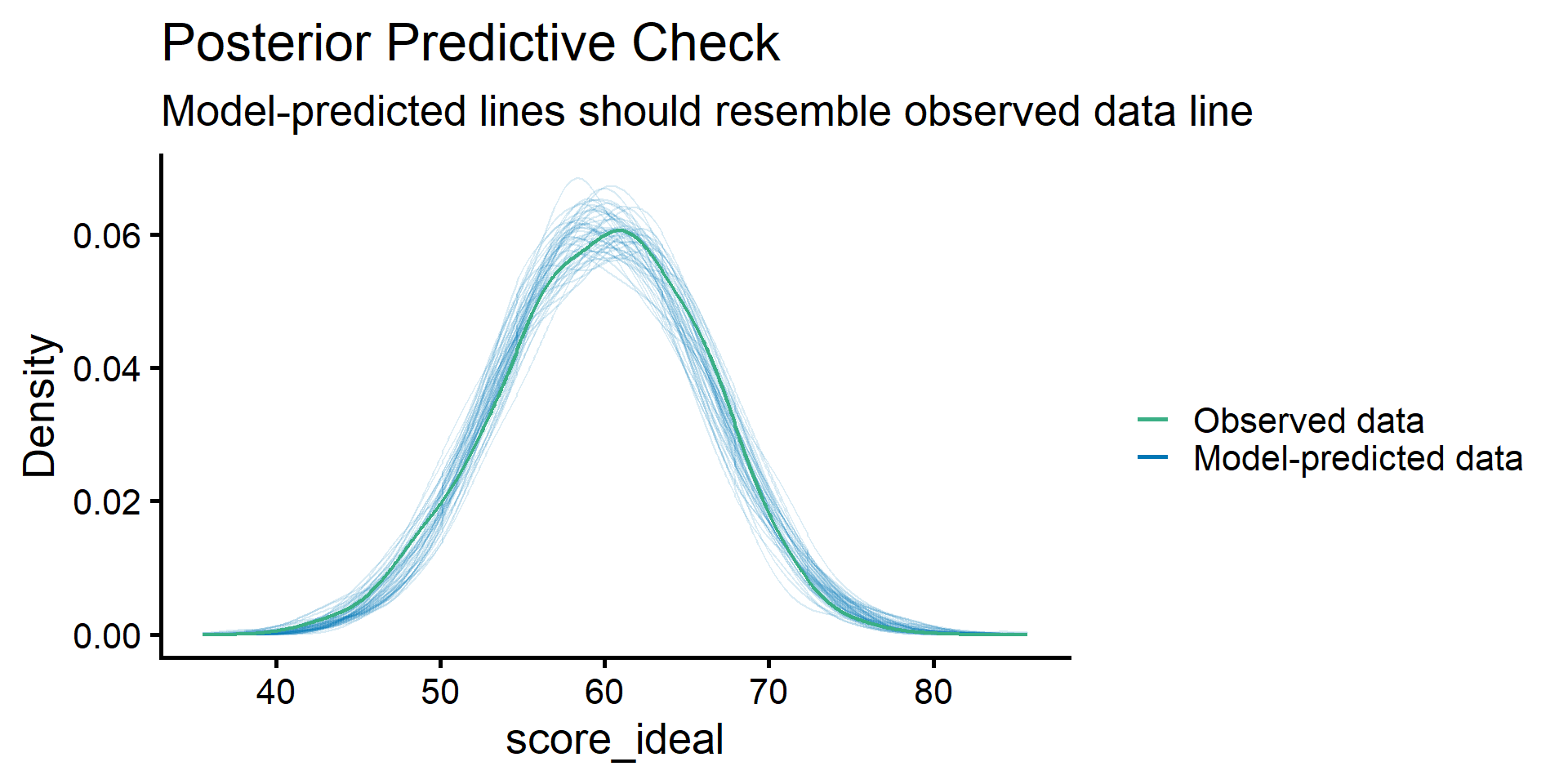
Before zooming in on residuals, we need to check the macroscopic fit of our model.
The check_predictions() function simulates new datasets based on your fitted model’s parameters and compares their overall shape to your actual data.
The Goal: If your model accurately reflects the true data-generating process, the simulated predictions (the blue lines) should overlap your raw data (the green line).

Plotting Predictions

check_predictions(fit_fixed)

Diagnosing Predictive Misfit

What if the model predictions do not align with the raw data? This indicates fundamental misspecification. No amount of residual tweaking will fix a model that cannot replicate the basic shape of your outcome.

Bimodal Data (Two humps): The model is only predicting one peak, but the data has two. You are likely missing a critical categorical predictor or grouping variable that separates the observations.
Skewed Data (Long tails): The model predicts a symmetrical curve, but the data has a long tail. You likely need to change the distribution family (e.g., moving to a Gamma or Poisson distribution) or apply a transformation.
Shifted Peaks: The model’s center is entirely offset from the data’s center. You might be missing important non-linear effects, such as polynomial terms or interactions.

Part 5: Residuals

1. Normality of Residuals

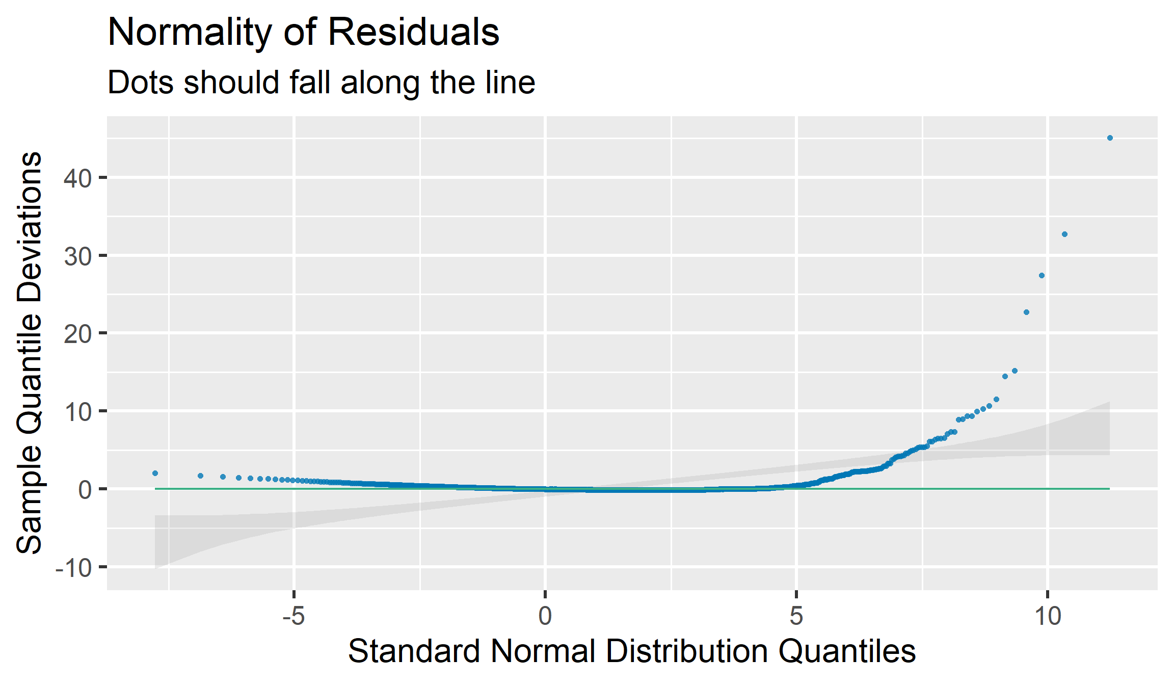
fit_skew <- glmmTMB(score_skew ~ homework + (1 + homework | school), data = dat)
check_normality(fit_skew, effects = "fixed") |> plot()

Interpreting Residual Normality

This plot checks the Level 1 errors (\(\color{#4daf4a}{e_{ij}}\)).
The points should fall tightly along the green reference line.
If points drift heavily at the tails, your residuals are skewed or heavy-tailed. Severe deviations here can bias your standard errors and \(p\)-values.

2. Normality of Random Effects

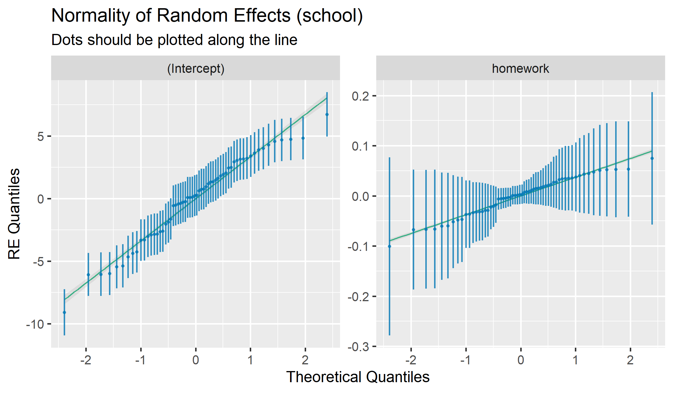
check_normality(fit_skew, effects = "random") |> plot()

Interpreting RE Normality

This plot checks if the cluster-level deviations (\(\color{#e41a1c}{u_j}\)) follow a normal distribution.
Each dot represents a specific cluster (e.g., a school).
Extreme deviations here mean certain clusters behave completely differently than the rest of the population, which might require investigation.

3. Homogeneity of Variance

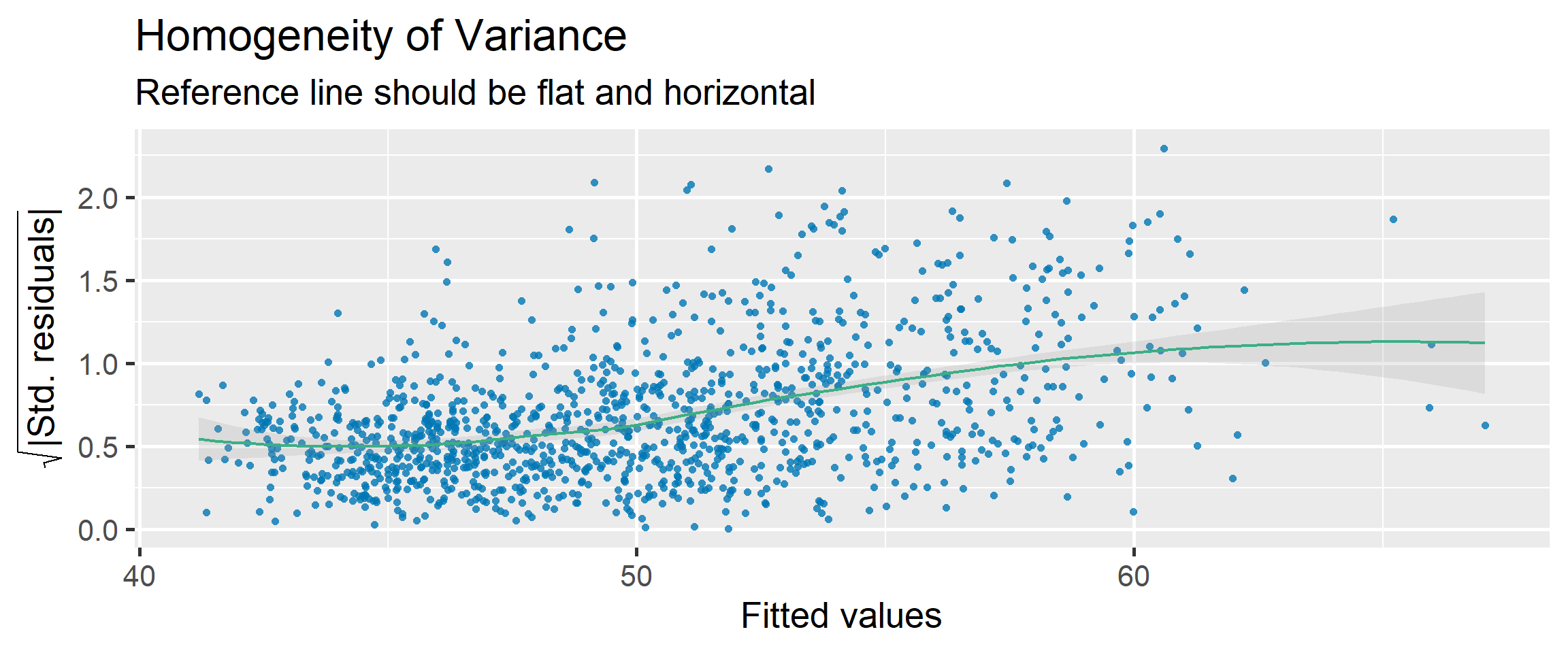
fit_het <- glmmTMB(score_het ~ homework + (1 + homework | school), data = dat)
check_heteroskedasticity(fit_het) |> plot()

Interpreting Homogeneity

The green reference line should be relatively flat and horizontal.
If the line bends sharply or the points fan out (like a megaphone), the variance is not constant (\(\color{#4daf4a}{\sigma}\) is changing).
In this plot, we can clearly see the variance expanding as the fitted values increase.

Fix: Modeling Variance Directly

If variance is not constant, we can actually model why it changes. The glmmTMB package allows us to predict the variance (\(\sigma\)) just like we predict the mean using the dispformula argument.

# Modeling variance as a function of homework
fit_disp <- glmmTMB(
  score_het ~ homework + (1 | school),
  dispformula = ~ homework, 
  data = dat
)

(Note: This creates a Location–Scale Mixed Model, where we estimate slopes for both the average and spread of the scores).

Part 6: Outliers

Outliers in MLMs

In standard regression, an outlier just pulls the line
In MLMs, outliers distort our system of variances
L1 Outlier (\(\color{#4daf4a}{e_{ij}}\)): An observation that is extreme within its cluster.
- Impact: Inflates the residual variance (\(\color{#4daf4a}{\sigma}\)), making all standard errors larger and reducing your power to detect true effects.
L2 Outlier (\(\color{#e41a1c}{u_j}\)): A cluster that is extreme among clusters.
- Impact: Distorts the main fixed effects (slopes) and inflates cluster variance (\(\color{#e41a1c}{\tau}\)), making groups look more different than they actually are.

Why DHARMa for Outliers?

The Problem with Traditional Outlier Metrics: Tools like Cook’s Distance struggle in MLMs because the model intentionally “shrinks” extreme cluster estimates toward the mean.
Thus, check_outliers() does not yet support glmmTMB models.
The Simulation Solution: DHARMa bypasses this by simulating thousands of new datasets directly from your fitted model parameters.
Flagging Outliers: If a real data point falls completely outside the expected boundaries of those simulations, it is flagged as a structural outlier.

Identifying Outliers

library(DHARMa)
fit_out <- glmmTMB(score_outlier ~ homework + (1 | school), data = dat)
res_out <- simulateResiduals(fit_out)
testOutliers(res_out)


    DHARMa outlier test based on exact binomial test with approximate
    expectations

data:  res_out
outliers at both margin(s) = 5, observations = 1200, p-value =
0.1896
alternative hypothesis: true probability of success is not equal to 0.007968127
95 percent confidence interval:
 0.001354247 0.009696618
sample estimates:
frequency of outliers (expected: 0.00796812749003984 ) 
                                           0.004166667

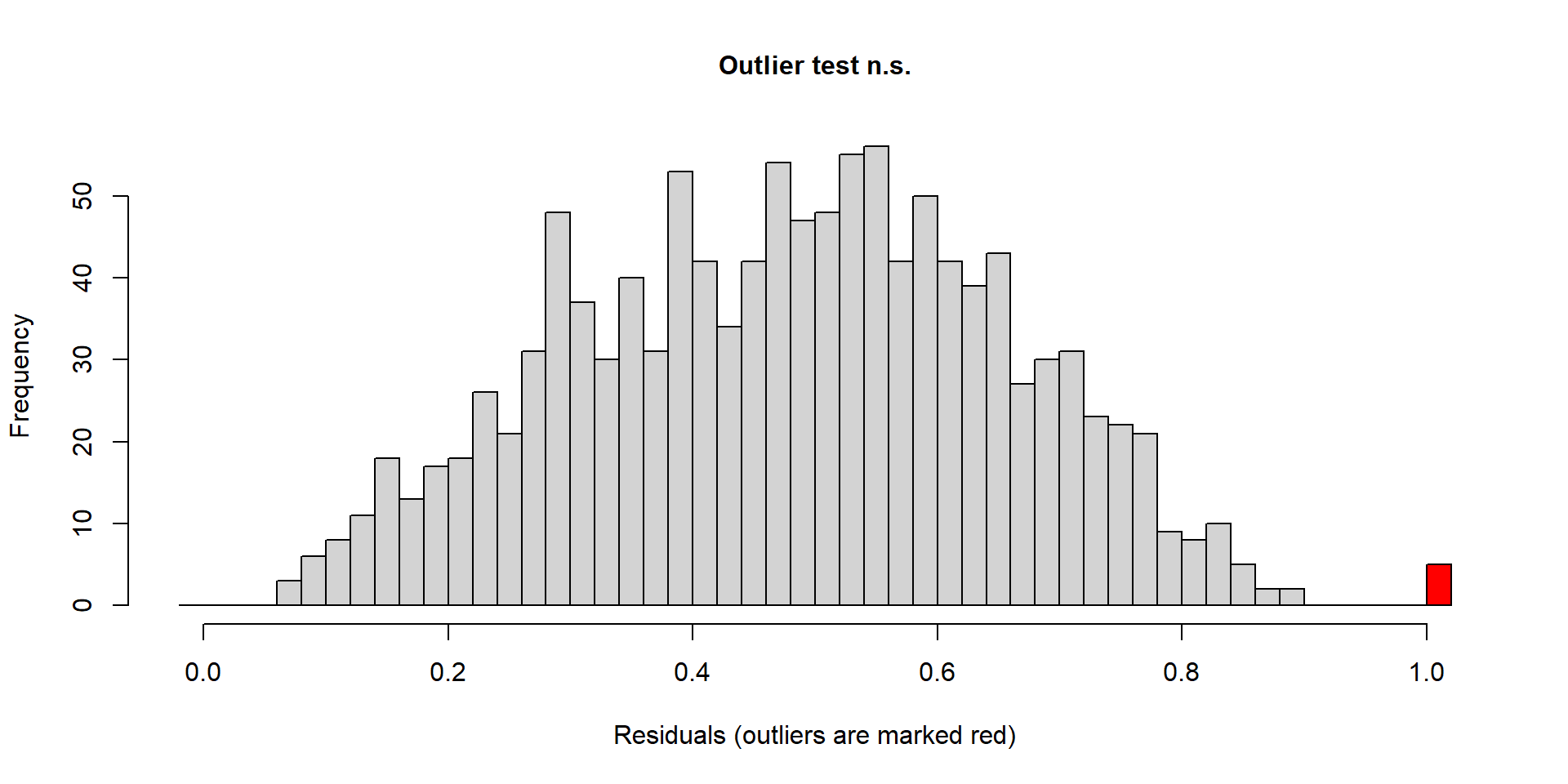
Plotting Outliers

Interpreting DHARMa Outliers

The Histogram: This plots your residuals as percentiles, not raw mathematical errors. Because a perfect model means a data point is equally likely to fall into any percentile, we want to see a flat, uniform block from 0.0 to 1.0, not a traditional bell curve.
The Red Bars: DHARMa assigns a value of exactly 0 or 1 to any data point that falls completely outside the simulated boundaries. These extreme outliers are grouped and highlighted in red at the very edges.
The Title: The title “Outlier test n.s.” means the test is “not significant.” Even though there is a red bar, the number of outliers is completely normal and expected for a dataset of this size.

Fix: Sensitivity Analysis

There is no magical R function to automatically “fix” outliers. You must use logic.

Identify the outliers using DHARMa.
Run the model with them.
Run the model without them.
Compare: If the main slope changes drastically, the outlier is “influential” and the results from both models should be reported transparently.

Performing the Sensitivity Analysis

To run the model without outliers, we first need to extract them. DHARMa flags outliers by assigning them a simulated residual of exactly 0 or 1.

# 1. Get the row numbers of the outliers
outlier_idx <- which(res_out$scaledResiduals %in% c(0, 1))

# 2. Create a clean dataset by dropping those rows
dat_clean <- dat |> slice(-outlier_idx)

# 3. Re-run the model on the clean data
fit_clean <- glmmTMB(score_outlier ~ homework + (1 | school), data = dat_clean)

Comparing the Results

Now we use compare_parameters() from the easystats package to look at both models side-by-side.

compare_parameters(fit_out, fit_clean, select = "{estimate} ({p})")

Parameter    |        fit_out |      fit_clean
----------------------------------------------
(Intercept)  | 54.87 (<0.001) | 53.93 (<0.001)
homework     |  1.15 (<0.001) |  1.21 (<0.001)
----------------------------------------------
Observations |           1200 |           1195

Interpreting the Comparison

Notice what happened to our slope for homework.

With Outliers: The effect of homework was severely underestimated (e.g., heavily pulled by the extreme points).
Without Outliers: The effect of homework recovered to its true value (closer to our simulated 1.2).
Conclusion: These outliers are highly influential. You should report the results of the clean model but be completely transparent in your manuscript about how many outliers were removed and why.