
“Which ICC should I report?” is the question this package is built to answer. There is no single intraclass correlation. The name hides a whole family of coefficients, and they do not all measure the same thing. In the jargon, they target different estimands: different true quantities you could be trying to pin down. The Glossary defines this and the other terms as they arise. Report the wrong one and you can overstate reliability by a wide margin. Or you can penalize a rating procedure for differences that do not actually matter to you.
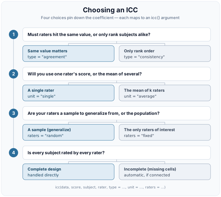
The good news: you do not need the formulas. You need to answer a few
plain questions about your study. Does the exact value matter,
or only the ranking? Will you use one rater or an average of several?
Each answer sets one argument of icc(). Four such choices
pin down the coefficient. Each is a genuine decision about your
measurement, not a technicality. Work through them top to bottom on the
single dataset below, so the numbers stay comparable. By the end you
will know both which coefficient to report and the exact call that
computes it.
The data
ratings is the six-subject, four-rater example of Shrout
and Fleiss (1979), in the long, one-row-per-rating format
icc() expects. Every subject is rated by every rater. So it
is a complete, balanced two-way design: each rater is
tracked across the subjects they score, and every cell is filled. That
is the clean case in which the choices below are easiest to see.
str(ratings)
#> 'data.frame':    24 obs. of  3 variables:
#>  $ subject: Factor w/ 6 levels "1","2","3","4",..: 1 2 3 4 5 6 1 2 3 4 ...
#>  $ rater  : Factor w/ 4 levels "1","2","3","4": 1 1 1 1 1 1 2 2 2 2 ...
#>  $ score  : num  9 6 8 7 10 6 2 1 4 1 ...
A prior question: are the raters crossed? (model)
Do the same raters score more than one subject, or
does each subject get a different set? If each rater is tracked
across the subjects they score, the design is crossed, like
ratings. Keep the default model = "twoway",
and the four choices below apply. Suppose instead each subject is rated
by whichever raters happened to be available. Then “rater 1” for one
subject has nothing to do with “rater 1” for another. Those raters are
interchangeable, and the design is one-way
(model = "oneway").
oneway <- icc(ratings, score, subject, rater, model = "oneway", seed = 2024)
oneway
#> ── Intraclass correlation: one-way random ──────────────────────────────────────
#> Subjects: 6 | Ratings: 24 (4 per subject, balanced) | raters interchangeable
#> Engine: glmmTMB (REML) | CI: 95% montecarlo (10000 draws)
#>
#>   index     estimate   95% CI
#>   ICC(1)       0.166   [0.008, 0.832]
#>   ICC(k)       0.443   [0.032, 0.952]
#>
#> Variance components: subject 1.244, residual 6.264 (rater confounded)
#> Shrout & Fleiss equivalent: ICC(1) = ICC(1,1), ICC(k) = ICC(1,k)
A one-way model cannot separate systematic rater differences from
error. So it folds them into the residual and reports a single
ICC(1) / ICC(k). That makes it the
most conservative coefficient. On this data
ICC(1) is 0.17, below the two-way ICC(A,1) and
ICC(C,1) you will see next. The reason is that those two
separate the rater effect that one-way absorbs. The type
and raters choices below do not apply to one-way, where
there is no rater term to reason about. Answer this question first.
1. Must the values match, or only the order?
(type)
Does the actual value need to match, or only the rank order? Absolute agreement means raters give the same score. It treats a systematic difference between raters, one judge scoring consistently higher than another, as error. Consistency asks only that raters agree apart from a constant offset per rater.
agreement <- icc(ratings, score, subject, rater, type = "agreement", seed = 2024)
agreement
#> ── Intraclass correlation: two-way random, absolute agreement ──────────────────
#> Subjects: 6 | Raters: 4 (random) | Observations: 24 of 24 cells (complete)
#> Engine: glmmTMB (REML) | CI: 95% montecarlo (10000 draws)
#>
#>   index     estimate   95% CI
#>   ICC(A,1)     0.290   [0.050, 0.713]
#>   ICC(A,k)     0.620   [0.173, 0.909]
#>
#> Variance components: subject 2.556, rater 5.244, residual 1.019
#> Shrout & Fleiss equivalent: ICC(A,1) = ICC(2,1), ICC(A,k) = ICC(2,k)

consistency <- icc(ratings, score, subject, rater, type = "consistency", seed = 2024)
consistency
#> ── Intraclass correlation: two-way random, consistency ─────────────────────────
#> Subjects: 6 | Raters: 4 (random) | Observations: 24 of 24 cells (complete)
#> Engine: glmmTMB (REML) | CI: 95% montecarlo (10000 draws)
#>
#>   index     estimate   95% CI
#>   ICC(C,1)     0.715   [0.343, 0.924]
#>   ICC(C,k)     0.909   [0.676, 0.980]
#>
#> Variance components: subject 2.556, rater 5.244, residual 1.019
Here ICC(A,1) is 0.29 but ICC(C,1) is 0.71.
The gap is not noise. It is a direct read-out of how much the raters
differ in average level. Consistency is never smaller than agreement,
because it drops a source of error. Choose agreement
when the number itself must be trusted (a clinical score, a physical
measurement). Choose consistency when only relative
standing matters (ranking applicants).
2. Single vs. average (unit)
Will you use one rater’s score, or the mean of
several? icc() returns both rows by default.
ICC(*,1) is a single-rater coefficient, the reliability of
one rater’s score. ICC(*,k) is an average-rater
coefficient, the reliability of a mean of several raters, here your
k raters. Averaging cancels independent error, so
ICC(*,k) is always the larger number (the Spearman–Brown
relationship).
For absolute agreement above, the single-rater 0.29 rises to 0.62 for
the four-rater mean. Report ICC(*,k) only if the averaged
score is what you will actually act on. If downstream users see one
rater’s judgment, ICC(*,1) is the honest figure. Request
one or both with unit = "single",
unit = "average", or the default
c("single", "average").
3. A sample of raters, or the only raters?
(raters)
Are your raters a sample you want to generalize beyond, or the entire population of interest? Random raters (the default) are a sample, and the coefficient generalizes to the rater universe they were drawn from. Raters are fixed when the observed raters are the whole population of interest. Then the coefficient does not generalize past them.
fixed <- icc(ratings, score, subject, rater, raters = "fixed", seed = 2024)
#> Warning: Modeling raters as fixed restricts inference to exactly these raters. You
#> cannot generalize to other raters.
#> ℹ For interrater reliability, the two-way random model (`raters = "random"`) is
#>   the recommended default (ten Hove et al. 2024; McGraw & Wong 1996, Case 2).
#> ℹ Use "fixed" only when these are the entire population of raters you will ever
#>   use.
icc() warns on raters = "fixed" because
random is the recommended default for interrater reliability: fixing the
raters answers a narrower question. On this balanced
design the fixed and random point estimates coincide. But they
are fit by different models, and their intervals differ. On
incomplete data even the point estimates diverge, as
shown below. Prefer random unless you truly never
intend to generalize beyond these exact raters.
4. Complete vs. incomplete designs
Is every subject rated by every rater? When cells
are missing, the classical ANOVA identities break down. The mixed model
icc() fits does not: it uses whatever ratings are present.
Two things change automatically:
- The design must stay connected, meaning the raters
and subjects form one linked web. A disconnected design cannot separate
subject from rater variance. So
icc()fails loudly rather than returning a plausible-looking number. - The averaging divisor for
ICC(*,k)becomesk_eff.k_effis the effective number of ratings: the harmonic mean of the per-subject rating counts, an average that leans toward the smaller values. So a few well-rated subjects cannot disguise the many that were rated by fewer raters. It honestly reflects the ragged averages you actually computed.
A worked incomplete design
ratings_incomplete is ratings with one
change: rater 2 acted as a pilot and scored only the first two subjects,
leaving four empty cells.
inc <- icc(ratings_incomplete, score, subject, rater, seed = 2024)
inc
#> ── Intraclass correlation: two-way random, absolute agreement & consistency ────
#> Subjects: 6 | Raters: 4 (random) | Observations: 20 of 24 cells (incomplete)
#> Engine: glmmTMB (REML) | CI: 95% montecarlo (10000 draws)
#>
#>   index     estimate   95% CI
#>   Absolute agreement
#>   ICC(A,1)     0.249   [0.038, 0.693]
#>   ICC(A,k)     0.521   [0.114, 0.881]
#>   Consistency
#>   ICC(C,1)     0.629   [0.228, 0.906]
#>   ICC(C,k)     0.847   [0.491, 0.969]
#>
#> ICC(*,k) projects to an effective 3.27 raters (harmonic mean of ratings/subject).
#> Variance components: subject 2.281, rater 5.532, residual 1.344
#> Shrout & Fleiss equivalent: ICC(A,1) = ICC(2,1), ICC(A,k) = ICC(2,k)
The header now reads 20 of 24 cells (incomplete).
ICC(*,k) now averages over an effective 3.27
raters rather than 4, the harmonic mean of the per-subject counts. Four
subjects were seen by three raters, two by all four. The estimate sits a
little below the complete-data value, as fewer ratings warrant.
Fixed and random now diverge
On the balanced ratings, raters = "fixed"
and raters = "random" returned the same point estimate. On
incomplete data they no longer do. They are different models, and the
missing cells give them different information about the rater
effects.
random_inc <- tidy(icc(ratings_incomplete, score, subject, rater,
  raters = "random", seed = 2024))
fixed_inc <- suppressWarnings(tidy(icc(ratings_incomplete, score, subject, rater,
raters = "fixed", seed = 2024)))| Random and fixed raters on ratings_incomplete | |||
| Coefficient | Estimate | 95% interval, lower | 95% interval, upper |
|---|---|---|---|
| Random raters | |||
| ICC(A,1) | 0.249 | 0.038 | 0.693 |
| ICC(A,k) | 0.521 | 0.114 | 0.881 |
| ICC(C,1) | 0.629 | 0.228 | 0.906 |
| ICC(C,k) | 0.847 | 0.491 | 0.969 |
| Fixed raters | |||
| ICC(A,1) | 0.236 | 0.057 | 0.630 |
| ICC(A,k) | 0.503 | 0.166 | 0.848 |
| ICC(C,1) | 0.621 | 0.218 | 0.906 |
| ICC(C,k) | 0.843 | 0.477 | 0.969 |
For the agreement coefficients, the random interval is the wider of the two. The consistency intervals, which leave out rater differences, stay close. Generalizing to a rater universe carries the extra uncertainty of which raters you happened to sample. Fixing the raters removes that uncertainty from the agreement coefficients. So the choice matters more once data are incomplete.
When a design is not identified
Connectedness is not a formality. Suppose the raters split into
groups that never share subjects. Then a subject difference cannot be
told apart from a rater difference, and icc() stops rather
than returning a plausible-looking number:
disconnected <- data.frame(
  subject = factor(c(1, 1, 2, 2, 3, 3, 4, 4)),
  rater = factor(c(1, 2, 1, 2, 3, 4, 3, 4)),
  score = c(5, 6, 4, 5, 7, 8, 6, 7)
)
icc(disconnected, score, subject, rater)
#> Error in `icc()`:
#> ! The subject-by-rater design is disconnected, so the subject and rater
#>   variances cannot be separated.
#> ℹ Every subject and rater must be linked through shared ratings (one connected
#>   design).
#> ℹ For unlinked rater groups, a one-way ICC (`model = "oneway"`) or additional
#>   linking ratings are needed.
Subjects 1–2 are rated only by raters 1–2, and subjects 3–4 only by raters 3–4: two islands with no bridge between them. This is exactly the ill-posed case the package refuses to guess at.
A fifth choice: subjects or clusters
Everything above takes the subject as the object of measurement.
Subjects may themselves be nested in higher-level units, such as pupils
within classrooms or patients within clinics. Then you may instead want
the reliability of the cluster mean, a multilevel ICC (ten
Hove, Jorgensen & van der Ark, 2022). Pass a cluster
column to icc(). It then reports two coefficients, where
the subject level is reliability within a cluster, and
the cluster level is reliability of cluster means. The
subject level asks how reliably raters distinguish subjects within a
cluster, and the cluster level asks the same of cluster means. The Multilevel designs article
works a full example.
Once you have a number
Picking the right coefficient is one half of the work. Reading it is the other half. Two habits keep you honest, whichever coefficient you chose. Interpret it against its confidence interval, not the point estimate alone. A small study can leave the reliability genuinely uncertain across a wide range. And treat published “poor / good / excellent” cutoffs as rough conventions, not verdicts. The bar that matters depends on the stakes of your decision and on which coefficient you are reading. The Getting started article’s “Is this a good ICC?” section lays out the common rules of thumb and their caveats.
Naming crosswalk
Two older naming schemes are still common. icc() prints
both its own McGraw–Wong label and, where one exists, the Shrout–Fleiss
number:
Your choice (type × raters) |
McGraw & Wong (1996) | Shrout & Fleiss (1979) |
|---|---|---|
| agreement × random |
ICC(A,1), ICC(A,k)
|
ICC(2,1), ICC(2,k)
|
| consistency × fixed |
ICC(C,1), ICC(C,k)
|
ICC(3,1), ICC(3,k)
|
| consistency × random |
ICC(C,1), ICC(C,k)
|
(no classic name) |
| agreement × fixed |
ICC(A,1), ICC(A,k)
|
(no classic name) |
The two off-diagonal rows are worth noticing. The classic
Shrout–Fleiss triplet
ICC(1,·)/ICC(2,·)/ICC(3,·) never
named a two-way random consistency or a two-way fixed
absolute-agreement coefficient. Both are perfectly well-defined
estimands that icc() computes.
Or let the package choose
Would you rather answer the questions than remember which argument
each maps to? choose_icc() walks the same tree. It hands
back the coefficient or coefficients to report, together with the exact
icc() call that computes them. It does not
fit anything, and it takes no data argument. So it is a
quick way to settle the choice before you run the model.
choose_icc(type = "agreement", unit = "single", raters = "random")
#> ── Recommended ICC ─────────────────────────────────────────────────────────────
#> Design: two-way random, absolute agreement
#>
#> Recommendation: ICC(A,1)
#> Shrout & Fleiss equivalent: ICC(A,1) = ICC(2,1)
#>
#> Why:
#>   - Crossed (two-way): each rater is tracked across the subjects they score.
#>   - Absolute agreement: the value itself must match. A systematic difference between raters counts as error.
#>   - Single rater: you will act on one rater's score.
#>   - Random raters: a sample you generalize beyond, to the rater universe they were drawn from.
#>
#> Run this on your data:
#>   icc(data, score, subject, rater, type = "agreement", unit = "single")
#>
#> Notes:
#>   - Complete vs. incomplete is automatic: icc() uses whatever ratings are present and projects ICC(*,k) to the effective number of ratings (k_eff). The design must stay connected, or icc() fails loudly.
Pass the decisions as arguments, as above. Or, in an interactive
session, call choose_icc() with them omitted to be asked
each outstanding question in turn. The type,
unit and level questions each also take
"both", which asks for the pair rather than making you
choose one. Answering a choice that does not apply to your design is a
clear error rather than a silent guess. One example is type
under a one-way model.
Summary
Pick agreement vs. consistency by whether the value
or only the rank must match. Pick single vs. average by
how many raters you will actually use. Pick random
vs. fixed by whether you generalize beyond these raters. Let
icc() handle complete vs. incomplete for
you, provided the design stays connected.
References
McGraw, K. O., & Wong, S. P. (1996). Forming inferences about some intraclass correlation coefficients. Psychological Methods, 1(1), 30–46.
Shrout, P. E., & Fleiss, J. L. (1979). Intraclass correlations: Uses in assessing rater reliability. Psychological Bulletin, 86(2), 420–428.
ten Hove, D., Jorgensen, T. D., & van der Ark, L. A. (2022). Interrater reliability for multilevel data: A generalizability theory approach. Psychological Methods, 27(4), 650–666.