Intraclass correlation coefficient for a two-way design

Estimates interrater-reliability intraclass correlation coefficients (ICCs) from a fitted linear mixed model, rather than from classical ANOVA mean squares. icc() computes the two-way absolute-agreement (ICC(A,*)) or consistency (ICC(C,*)) coefficients of McGraw & Wong (1996). It reports them for a single rater (ICC(*,1)) or the mean of k raters (ICC(*,k)), treating the raters as a random sample (Case 2) or as fixed (Case 3).

Usage

autoplot.icc(object, what = "coefficients", ...)

# S3 method for class 'icc'
plot(x, ...)

# S3 method for class 'icc'
format(x, ...)

# S3 method for class 'icc'
print(x, ...)

# S3 method for class 'icc'
summary(object, ...)

# S3 method for class 'icc'
tidy(x, ...)

# S3 method for class 'icc'
glance(x, ...)

icc(
  data,
  score,
  subject,
  rater,
  cluster = NULL,
  model = "twoway",
  type = c("agreement", "consistency"),
  raters = "random",
  unit = c("single", "average"),
  occasions = "single",
  level = c("subject", "cluster"),
  design = NULL,
  engine = "glmmTMB",
  conf_level = 0.95,
  ci_method = "montecarlo",
  mc_samples = 10000L,
  boot_samples = 999L,
  seed = NULL,
  brm_args = list(),
  prior = NULL,
  posterior_summary = "percentile"
)

Arguments

what

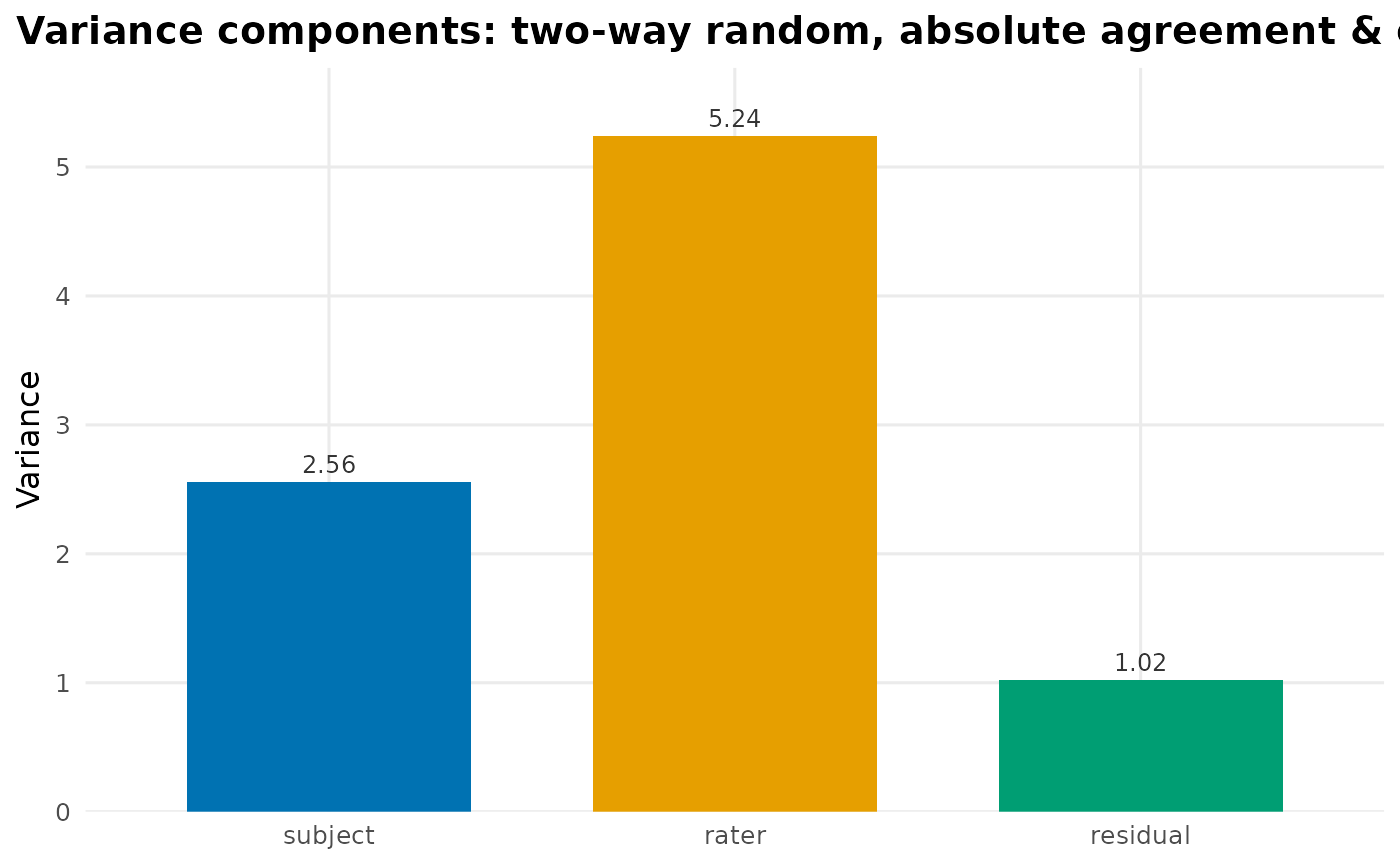
Which plot to draw: "coefficients" (the default) for a forest plot of each ICC index with its Monte-Carlo confidence interval, or "components" for the variance-component decomposition.

...

Unused, for method consistency.

x, object

An icc object.

data

A data frame with one rating per row.

score, subject, rater

Columns of data (unquoted): the numeric rating, the subject (object of measurement), and the rater (judge). A non-finite score (Inf, -Inf, NaN) is an error. An NA score is treated as a rating that did not happen. The row is dropped with a suppressible intraclass_dropped_rows warning, and the rest is analyzed as an incomplete design, so a missing rating and an absent row give the same answer.

cluster

Optional column of data (unquoted) giving the higher-level unit each subject is nested in (e.g. classroom, clinic). Supplying it switches on the multilevel ICC (ten Hove et al. 2022). Reliability is reported at the subject and/or cluster level. See level and the Multilevel designs section. Left NULL (the default) for an ordinary single-level two-way ICC.

model

Design: "twoway" (the default, subjects crossed with a common set of raters) or "oneway" (each subject rated by a possibly different set of raters). Under "oneway" (Shrout & Fleiss Case 1) the raters are treated as interchangeable. In that design the rater column is used only to count the ratings per subject, and its labels are ignored. That design has no rater main effect to model, so type does not apply and the coefficients are ICC(1) / ICC(k). Fixed raters and a cluster (multilevel) structure are not defined for a one-way design.

type

Error definition(s) (two-way only): "agreement" (absolute agreement) counts systematic rater differences as error, and "consistency" ignores them. Like unit and level, type is vectorized and defaults to both (c("agreement", "consistency")). So a default call reports every defined formulation from the single fit: ICC(A,1), ICC(A,k), ICC(C,1), and ICC(C,k). Agreement vs. consistency is post-fit arithmetic on the same variance components, so the second definition is free. Pass a single value to report just that coefficient once you have named your estimand. A definition that is undefined for the design (e.g. "consistency" for a Design-3 nested-in-subjects fit, or a fixed-rater agreement projection to a different rater count) is dropped with a message when reached via the default, and aborts with a teaching error when requested explicitly. Not applicable when model = "oneway".

raters

Rater sampling. "random" (the default, two-way random, Case 2) generalizes to a rater universe. "fixed" (two-way mixed, Case 3) treats the observed raters as the entire population and is fit with raters as fixed effects (score ~ 1 + rater + (1 | subject)). On balanced data the point estimate matches "random". On incomplete data the two genuinely differ. Even when balanced, the interval differs for absolute agreement, because inference about fixed vs. random rater effects is not the same. Choosing "fixed" emits a warning, because random is the recommended default for interrater reliability.

unit

The averaging unit(s): "single" (-> ICC(*,1)), "average" (-> ICC(*,k)), or a number m >= 1 for a D-study projection to the mean of m raters (-> ICC(*,m)), or any combination. See d_study() for projecting across a range of m. Projecting absolute agreement is not defined for fixed raters (see d_study()).

occasions

For data with within-cell replicates (more than one rating per subject-by-rater cell), whether to average over them. Ask for "single", the reliability of one rating, and/or "average", the mean of the n_o replicates, which reduces pure error. "single" is the default and "average" requires replicated data. See the Within-cell replicates section. Ignored with one rating per cell.

level

For multilevel designs (a cluster column), which reliability to report: "subject" (within-cluster, distinguishing subjects) and/or "cluster" (between-cluster, distinguishing cluster means). Defaults to both. "conflated" may be added for the biased ignore-the-clustering ICC as a diagnostic contrast (crossed random-rater designs, balanced or incomplete). See the Multilevel designs section. Ignored (and must be left at its default) when cluster is not supplied. Only "subject" is available when raters are nested in clusters.

design

Multilevel design (with a cluster column). NULL (the default) infers it from the crossing pattern. There are two occasions to override that inference. The first is when the rater labels do not mean what the crossing pattern implies, as in a complete table whose rater labels repeat across clusters. The second is when missing cells leave the pattern genuinely ambiguous between a crossed and a nested design. Declare the design explicitly with "crossed", "nested_in_clusters", or "nested_in_subjects". A declaration is validated against the data, and cannot force a design the data cannot support (e.g. "crossed" still requires raters that bridge clusters to estimate absolute agreement).

engine

Estimation engine: "glmmTMB" (default), "lme4", "lavaan", or "brms". "glmmTMB" and "lme4" fit the variance components by REML and agree to within numerical tolerance on balanced data. "lavaan" fits the equivalent structural-equation (common-factor) generalizability model and recovers the rater main effect from the mean structure (Jorgensen 2021). Consistency ICCs from "lavaan" equal the mixed-model estimates exactly on balanced data. Absolute-agreement ICCs from "lavaan" use the SEM indicator-mean estimator of the rater variance. That estimator is asymptotically equivalent to the mixed-model one and matches conventional generalizability-theory software on real data (Vispoel et al. 2022). But it differs by a small-sample term on tiny designs, e.g. 0.284 vs 0.290 on the 6-subject example below. "lme4" covers every design "glmmTMB" does: two-way (random or fixed raters), one-way, and the multilevel designs (crossed and nested) at both levels. It covers them on both balanced and incomplete/ragged data. A ragged fit that lands exactly on a variance-component boundary falls back to "glmmTMB" (which stays finite via its log-SD parameterization) with a clear message. "lavaan" covers the two-way design with random or fixed raters, on both complete and incomplete data. For fixed raters the agreement rater term is the McGraw & Wong Case-3A bias-corrected finite-population variance, which equals the mixed-model estimate on balanced data. In the two-way SEM, with either rater type, missing cells are estimated by full-information maximum likelihood, and the parametric bootstrap is unavailable for incomplete SEM. It also covers the crossed (Design 1) multilevel design at both levels, plus the conflated diagnostic, via a two-level SEM. With random raters the multilevel fit covers complete/balanced data. It also covers incomplete data (missing cells estimated by two-level full-information ML) and unbalanced data (unequal cluster sizes). For that random-rater two-level fit the interval is the Monte-Carlo interval (the default). Its parametric bootstrap, which simulates two-level datasets from the fitted moments and refits per resample, is available on balanced/complete data only. For that fit, incomplete or unbalanced data is Monte-Carlo only, because resamples cannot reproduce a missingness pattern and the bootstrap coverage is validated only on balanced data. With fixed raters the between-level rater intercepts give the Case-3A finite-population \(\theta^2_r\) at both levels, on complete, balanced data with equal cluster sizes only. That path is Monte-Carlo only: its fixed-rater bootstrap is not yet available. Because lavaan's random-rater term is the raw quadratic form, the fixed-rater ICC differs from the random-rater one by the finite-population correction, which the REML-based mixed-model engines do not carry into their random estimate. lavaan's two-level estimator is full-information ML, and there is no REML analog. So with few clusters its cluster-level components sit slightly below the REML estimates, and its absolute-agreement rater term slightly above. Both differences shrink as clusters grow. Its consistency ICCs are ratios, so they agree with the mixed-model estimates essentially exactly. "brms" fits the random-rater model in a Bayesian framework (Stan, via brms), under a sourced half-t(4, 0, 1) prior on the random-effect SDs (ten Hove et al. 2020). The point estimate is the posterior mode (MAP), and the interval is a percentile credible interval (ci_method = "posterior", forced). On both balanced/complete and incomplete/ragged data it covers the two-way random single-level design, and the crossed (Design 1) multilevel random design (subject and cluster levels). On that same data it covers the two-way fixed-rater single-level design (Case-3A finite-population \(\theta^2_r\)), and the crossed (Design 1) multilevel fixed-rater design (subject level). On that same data it also covers the nested Design 2 and Design 3 random multilevel designs at the subject level, and the single-level one-way random design. Design 2 nests raters in clusters. Design 3 nests them in subjects, which is the multilevel one-way, agreement-only case. The nested Design 2 fixed-rater multilevel design is covered at the subject level on both balanced and incomplete/ragged data. On balanced/complete data only it covers the crossed Design 1 fixed-rater cluster level, the conflated diagnostic, and within-cell replicates. Within-cell-replicate Bayesian fits and numeric-unit (D-study) projection are planned for later milestones. "lme4" requires the lme4 and merDeriv packages. "lavaan" requires the lavaan package. "brms" requires the brms package, and a working Stan toolchain.

conf_level

Confidence level for the interval (default 0.95). Any level in (0, 1) is accepted, except under ci_method = "mpl", which is calibrated at 0.90, 0.95, and 0.99 only. At each of those levels the between-node subject-count interpolation is coverage-checked (see ci_method).

ci_method

Interval method. "montecarlo" (default) simulates from the fitted parameter covariance on the engine's log scale (fast, boundary-aware). Near the variance boundary it can fail to produce an interval and aborts. When it does, the error names an opt-in method below that fits the design in hand. That method is chosen by RUNNING each candidate on your data, keeping only those whose reported endpoints are all finite, correctly ordered and in range. So there is no need to work that out from this list. Being a check on the data rather than on the design, it falls silent wherever a method would not in fact deliver. That includes degenerate data, an uncalibrated conf_level or geometry, and a numeric unit projected past the point where a method's Spearman-Brown map breaks down. The two closed forms are asked separately, so one can be named where the other is not. On unbalanced one-way data it can name "npbootstrap". Because that method resamples, its trial run is evidence about one run rather than about the data. So the trial uses your call's own boot_samples and your own seed when you set one, in which case your retry reproduces it exactly. With no seed set it uses a fixed seed the message then names, and an unseeded retry draws fresh resamples and can fail where the verified run succeeded, especially on small designs. The trial run leaves the session's random-number stream untouched. The same holds in reverse, and on "bootstrap", "searle", "burch" and "npbootstrap" as well as on the default ("mpl" raises its own kind of error and is not covered). When a method you asked for aborts on degenerate data, its error names a method verified on that same data by the same trial runs and under the same rules. Where no method serves that data it names none, leaving the message exactly as it would otherwise read. It never names the method you asked for, which just failed. Data with no between-subject variance is the case this matters most on: there "bootstrap" is typically the only method that returns anything usable, and it is now named rather than left for you to find. Candidates are tried cheapest first. So the two methods that reduce the fitted model rather than your raw data, "bootstrap" and "montecarlo", are reached only where no method fenced to your design serves the data. The costliest of them is both screened at a small resample count and capped when run in full, so an error stays a few seconds rather than tens of them. That cap is why a bullet naming "bootstrap" also names a boot_samples value. It is the count the trial actually ran at, and the call the message gives you is the one that was verified rather than a heavier one nobody tried. "bootstrap" is a parametric bootstrap: it simulates response vectors from the fitted model, refits, and takes percentile quantiles of the resampled coefficients. The bootstrap does not rely on the asymptotic-normal covariance approximation but is far slower (a refit per resample). It is available for every design the "glmmTMB" and "lme4" engines fit, via glmmTMB's simulate() + refit and lme4::bootMer respectively. It is also available on the "lavaan" engine, which simulates from the fitted SEM's implied moments and refits, for the random two-way design and the crossed (Design 1) random-rater multilevel design. As with the Monte-Carlo interval, the "lme4" engine defers a singular (boundary) fit to "glmmTMB" for either method. At the zero-between-subject-variance boundary the point estimate and the interval come from different computations. The point comes from the engine's REML fit, and the endpoints from quantiles of the refits, so the reported conf.low can sit slightly above the reported point instead of below it. Both numbers are zero to any reading when that happens: over every cell of the sweep committed at tests/testthat/fixtures/bootstrap-point-containment.tsv, each such gap and each such point estimate is below 1e-8. Nothing is clamped and no error is raised, and in that sweep's cells with real between-subject signal the interval contains its point. "posterior" is the percentile credible interval from the Bayesian engine's posterior draws. It is the forced default for, and available only with, engine = "brms", and "brms" requires it. The other methods do not apply to a Bayesian fit, and "posterior" needs posterior draws no other engine produces. "npbootstrap" is the non-parametric transformed bootstrap-t of Ukoumunne et al. (2003), for the one-way random design (model = "oneway", and it aborts otherwise). It serves both unit = "single" (ICC(1)) and unit = "average" (ICC(k)) on balanced and unbalanced data (unequal ratings per subject) alike. On unbalanced data the effective group size becomes the ANOVA n0 of Ohyama (2025). Only a numeric unit (a D-study projection to m raters) is restricted to balanced data. For a projection on unbalanced data, use ci_method = "montecarlo". It resamples whole subjects with replacement (not from the fitted model), stabilizes the variance with the log F transform, studentizes with an infinitesimal-jackknife SE, and back-transforms the endpoints. It is not a percentile bootstrap. The percentile and BCa variants were assessed and rejected, because they under-cover at small rater counts. Reach for it for its boundary robustness (an interval that exists where the Monte-Carlo default aborts) and non-normality robustness. See Details for the ICC(k), endpoint-support, and point-estimate conventions. "searle" and "burch" are two deterministic classical closed-form intervals, also only for the balanced one-way random design (they abort otherwise). Both return a finite interval at the near-zero-ICC boundary where the Monte-Carlo default aborts, with one asymmetry. On data with no between-subject variance at all, "burch" aborts (its kurtosis standardization divides by zero there) while "searle" still returns an interval. Read that interval carefully: the single-rater coefficient gets the attained minimum, while the averaged projection carries that minimum through the Spearman-Brown pole to -Inf, which a default call prints beside it. Neither resamples, so mc_samples, boot_samples, and seed do not apply. "searle" is the exact-F pivot (Searle 1971, Table 9.14; McGraw & Wong 1996, Table 7): exact under normality, and best-calibrated when the data are approximately normal. "burch" is the REML-based, kurtosis-adjusted interval of Burch (2011), designed for robustness to non-normality. Its width tracks the data's tail weight rather than widening by construction. On the two grids this package has measured that vary only the subject effect, "burch" is usually the narrower of the two. But the margin depends on the design, so it is not a rule of thumb. "burch"'s width margin holds much the same up to a true ICC of 0.3 rather than shrinking as the true ICC rises (on the larger grid; the smaller grid's margin does shrink across its levels). The margin then collapses to near parity at a true ICC of 0.6, on the one grid reaching that value, which is also where every cell "searle" won sits. And "burch"'s width margin shrinks steadily as the subject count grows, measured at 5 raters. What "burch" does against "searle" depends on what the residual is drawn from. The three grids now measure that: the two grids that vary only the subject effect put it narrower nearly everywhere, while the third, which draws the residual from the same family as the subject effect, puts it wider at every symmetric heavy-tailed family measured (a median width ratio of 1.2963 at t(5) with 100 subjects) and narrower at every lighter-tailed one, the normal included. Treat neither as reliably the tighter interval. The per-level figures for the two grids that vary only the subject effect are tabulated in the interval-methods article. Burch's robustness has limits this package has measured. On strongly skewed subject effects "burch" under-covers about as badly as the default, worst 0.6655 at chi-square(1) subject effects with a true ICC of 0.6, 30 subjects and 5 raters. Prefer "searle": across every distribution family in that study it landed closer to nominal coverage in most cells, including the heavy-tailed ones. "burch" dipped below the nominal level in fewer cells overall, which is the one respect in which it was steadier. But it is a remedy for neither heavy tails nor skew (see the coverage caveat under Confidence intervals). "mpl" is the modified profile-likelihood interval of Xiao & Liu (2013), only for the balanced-complete two-way random absolute-agreement ICC(A,1). ICC(A,k) and any numeric-unit projection ICC(A,m) are its Spearman-Brown image, pole-safe for every m >= 1. It aborts on any other design, on consistency (ICC(C,.)) or fixed raters, and on unbalanced or incomplete data. It is a deterministic closed form: no resampling, so mc_samples, boot_samples, and seed do not apply. Like "npbootstrap", it returns an interval at the near-zero-ICC boundary where the two-way Monte-Carlo default aborts. A limit is reported at the [0, 1] boundary only when the profile deviance shows the confidence set reaching it. A degenerate fit (raters in near-perfect agreement) or a failed root search raises a classed error rather than a fabricated boundary value. And it covers at or above nominal across the pre-registered grid where the incumbents can under-cover, assessed as GO-for-opt-in against that grid. It is deliberately conservative: it over-covers, and is wider than the Monte-Carlo interval at interior cells, so it is an opt-in, not the default.

Two constraints follow from its calibration. It is available only at conf_level 0.90, 0.95, or 0.99. The correction constant is calibrated separately at each level's own deviance quantile and is never interpolated between levels, so any other level aborts. And that constant is calibrated by simulation over rho in [0.05, 0.9], extending below Xiao & Liu's published rho >= 0.6 fence into a near-boundary region that carries no external oracle. There, and at conf_level = 0.99 throughout, its calibration rests on the package's own simulated coverage.

The constant's subject-count dimension is tabulated, not continuous. It is calibrated at subject-count nodes (10, 15, 20, 30, 50, and 100 subjects, per rater count and level) and linearly interpolated in the subject count between them. At a node the tabulated value is used exactly. The nodes are individually calibrated. The interpolated path is validated, not calibrated, by coverage probes at a handful of off-node geometries at each supported level. At the default 0.95 the validated cells are three: 3 raters with 25 subjects, and 10 and 2 raters with 40 subjects. All sit at one stress configuration (rater variance four times error variance, true ICC 0.60) in which only the rater and subject counts vary. Each clears the pre-registered 0.93 floor there. That floor is a nominal-minus-2-percentage-point tolerance, not at-or-above-nominal coverage: one validated cell measured 0.944. No validated cell pinned an endpoint at 0 or 1. And the one-sidedness described below is not uniform across rater counts. In the 3- and 10-rater cells misses fall mostly below the interval (31/2 and 42/14 of 1000 replicates), while the 2-rater cell missed only once, above. So an off-node subject count is safe to use at every supported level, but an asymmetry or width figure observed at one geometry must not be carried to another.

Two further characteristics are worth knowing before reporting an endpoint. The two-sided interval is not equal-tailed. Where rater variance is large relative to error and the subject count is high, non-coverage falls almost entirely on one side. In one validated cell 65 of 66 misses fell below the interval, not above. So a limit must not be read as a one-sided bound at half the complementary level. And at conf_level = 0.99 with very few raters the interval can be near-vacuous: median width 0.905 on the [0, 1] scale at 2 raters and 40 subjects. That is the honest cost of a deep tail at minimal rater information, not a defect (coverage there is 1.000), but such an interval excludes little. It assumes approximately Gaussian data (untested for non-normality).

mc_samples

Number of Monte-Carlo draws for ci_method = "montecarlo" (default 10000). It is also the count at which a "montecarlo" interval is trialled when some other method's error considers suggesting it.

boot_samples

Number of resamples for ci_method = "bootstrap" (the parametric bootstrap) and "npbootstrap" (the transformed bootstrap-t subject resamples), default 999. It does not change a ci_method = "montecarlo" interval, but it is not unused on that path: when that interval aborts, it is the count the suggestion machinery trials "bootstrap" at (capped) and names in the message.

seed

Optional integer seed for a reproducible interval (and, for engine = "brms", the Stan sampler seed). The global RNG state is restored afterward. It also seeds the trial runs behind an error's suggestion, so it can decide which method that error names, including for the deterministic "searle" and "burch" intervals, whose own values ignore it.

brm_args

A named list of extra arguments forwarded to brms::brm() when engine = "brms" (e.g. backend, chains, iter, cores, control). The default (rstan backend, brms defaults) needs none. By default brms samples the chains sequentially on one core (cores = getOption("mc.cores", 1L)). Pass brm_args = list(cores = 4), or set options(mc.cores), to sample in parallel. The engine emits a periodic reminder to that effect while running sequentially. The model formula, data, the sourced half-t prior, and seed are owned by intraclass and may not be set here. The prior has its own prior argument. Supplying them, or a non-empty brm_args with any other engine, is an error.

prior

Optional custom prior for engine = "brms", as a brms prior object (from brms::set_prior() or brms::prior()). Several priors can be combined with c(). The default NULL uses the sourced half-t(4, 0, 1) prior on every random-effect SD (ten Hove, Jorgensen & van der Ark 2020), the prior every coverage result in this package depends on. Supplying a custom prior is a deliberate deviation, intended for prior-sensitivity, method-comparison, or simulation work, and it voids those coverage guarantees. icc() warns loudly (a classed intraclass_custom_prior condition), because a vague or flat SD prior can worsen small-k boundary bias. The half-t is weakly informative on purpose. Ignored (must be NULL) for non-Bayesian engines.

posterior_summary

How to summarize the posterior draws into a credible interval when ci_method = "posterior" (the Bayesian engine): "percentile" (the default, a two-sided percentile interval) or "hpdi" (the highest-posterior-density interval, the narrowest interval covering the credible mass). Percentile is the default on several grounds. It is monotone-transformation invariant and degrades gracefully as the ICC approaches the variance boundary. And ten Hove, Jorgensen & van der Ark (2020) found percentile (not HPD) intervals give nominal coverage at small rater counts. The HPDI is offered for comparison, not as a strict upgrade, and no coverage is claimed for it. Only the HPDI needs the posterior draws, so posterior_summary = "hpdi" requires ci_method = "posterior". The other interval methods already report a percentile interval.

Value

icc() returns an icc object: a list with the estimate table, variance components, design, engine, interval settings, sample sizes, the fitted model, and the call.

What of that object is stable. The supported way to read a fit is through the methods below, plus two elements of the list itself: $fit, the object the engine returned, and $call, the matched call. Everything else in the list is internal: its names, nesting, and contents may change in any release without a deprecation cycle. That is the whole rule – $fit and $call are the list elements you may depend on, and reaching into any other one is reading an implementation detail. tidy() and glance() are the stable tables, not a re-export of the list: they report the estimated coefficients and the model-level summaries, column by column as documented below. Those two tables, plus $fit and $call, are the whole supported surface; everything else the list holds falls under the rule above, whether or not a table happens to report it.

The methods documented on this page return:

• tidy.icc(): a tibble with one row per estimated coefficient, columns in this order: term (the coefficient's ICC index, named for the broom glossary), occasions, type, level, sf_index, estimate, std.error, conf.low, conf.high, conf.level, method. Every column is present on every fit. occasions reports the per-rater occasion divisor that row's coefficient applies to pure error. On a fit that splits within-cell replicates it reads 1 wherever the row averages no occasions. That covers every single-occasion row, and every row whose error set carries no pure-error term to average, such as the cluster rows of a multilevel fit. It reads the fitted per-cell occasion count where the row does average. On a fit that splits none it is NA. It is not in general the number of ratings the coefficient averages, because it counts occasions per rater: an occasion-averaged ICC(*,k) row averages k raters at that occasion count each. glance() reports a different quantity as n_o, the observed per-cell occasion count of the fitted design. n_o is itself NA under the condition the glance.icc() bullet below states, which a ragged replicate design meets while occasions still reads 1.

• glance.icc(): a one-row tibble of model-level summaries: the sample sizes, the design flags – among them the rater treatment raters (NA where the design estimates no separable rater main effect: a model = "oneway" fit, whose raters are interchangeable and carry no facet, and a design = "nested_in_subjects" fit, whose rater effect is confounded into the residual) and replicates, whether the fitted design splits within-cell replicates – FALSE on a one-way fit, which has no rater facet and so no cells to split – the effective rater counts, the variance components, the occasion count n_o (NA unless the fitted design splits within-cell replicates and defines one occasion count per cell – the same number of ratings in every cell, and every cell the design defines present, which is the full subject-by-rater grid when crossed and the block-diagonal one when raters are nested in clusters; on a design failing either condition, n_o is reported as NA or the fit refused with an error, depending on the design), the engine and interval settings, and the sampler diagnostics rhat and ess_bulk (NA for the non-Bayesian engines, which do not sample). Every column is present on every fit, so two glanced fits row-bind just as two tidied ones do.

• format.icc(): a character vector holding the printed report, one line per element.

• print.icc(): the icc object invisibly, having emitted that report.

• summary.icc(): the icc object invisibly, having emitted the report followed by the interpretive notes.

• autoplot.icc(): a ggplot object holding the coefficient forest plot, or the variance-component decomposition when what = "components".

• plot.icc(): the icc object invisibly, having drawn that same plot.

tidy.icc() and glance.icc() implement the tidy() and glance() generics.

Which ICC is this, and when should you use it?

Three choices pin down the coefficient:

• Agreement vs. consistency (type). Absolute agreement treats systematic differences between raters (the rater main effect, \(\sigma^2_r\)) as error: use it when the actual value matters and raters must agree on the number (clinical scores, measurements). Consistency ignores a constant per-rater offset: use it when only relative standing matters. A large gap between the two signals big systematic differences in rater level, which is a rating-procedure problem worth fixing.

• Single vs. average (unit). ICC(*,1) is the reliability of a single rater, and ICC(*,k) is the reliability of the mean of your k raters. Report ICC(*,k) when the averaged score is what you will use.

• Random vs. fixed raters (raters). Random treats your raters as a sample you wish to generalize beyond, and is the recommended default for interrater reliability. Fixed treats them as the only raters of interest and forgoes generalization. It is fit separately, with raters as fixed effects, so on balanced data it matches the random point estimate but on incomplete data it genuinely differs. icc() warns when you choose it. Fixed-rater consistency is the classic Shrout & Fleiss ICC(3,1).

Estimand

With a single rating per subject-by-rater cell, the subject-by-rater interaction and pure error are not separately identified. In that case only their sum, the residual variance \(\sigma^2_{res}\), is estimable. Absolute agreement counts the rater main effect \(\sigma^2_r\) as error. Consistency drops it. $$ICC(A,1) = \sigma^2_s / (\sigma^2_s + \sigma^2_r + \sigma^2_{res})$$ $$ICC(A,k) = \sigma^2_s / (\sigma^2_s + (\sigma^2_r + \sigma^2_{res}) / k)$$ $$ICC(C,1) = \sigma^2_s / (\sigma^2_s + \sigma^2_{res})$$ $$ICC(C,k) = \sigma^2_s / (\sigma^2_s + \sigma^2_{res} / k)$$ Here \(\sigma^2_s\) is the subject (signal) variance and k is the number of raters.

Multilevel designs (subject vs. cluster level)

When subjects are nested in higher-level clusters (pupils in classrooms, patients in clinics), single-level ICCs conflate the levels and are biased (ten Hove et al. 2022). Supplying cluster fits the five-component Design-1 model $$score \sim 1 + (1|cluster) + (1|cluster{:}subject) + (1|rater) + (1|cluster{:}rater)$$ and reports two distinct reliabilities. The subject level (within-cluster) asks how reliably raters distinguish subjects within a cluster: its signal is the between-subject-within-cluster variance and cluster variance drops out. The cluster level (between-cluster) asks how reliably raters distinguish cluster means: its signal is the between-cluster variance and the rater-disagreement error is the cluster-by-rater term. Choose the level that matches the decision you will make (about a subject, or about a cluster). The agreement/consistency and single/average choices above apply at each level.

level = "conflated" reports the biased single-level ICC you would get by ignoring the clustering (ten Hove et al. 2022, Eq. 14). Between- and within-cluster subject variance are both counted as signal, and the rater-related terms as error. It is offered only as a diagnostic contrast, to quantify how much the nesting distorts reliability, and is never a recommended coefficient. print() flags it as such. It is the flat two-way ICC read off the multilevel fit, so it comes in both type forms: absolute agreement (Eq. 14) and consistency (which drops the rater main-effect variance, McGraw & Wong 1996). It needs a crossed (Design 1) random-rater design and works on both balanced and incomplete data (same k_eff divisor). Because it reads the cluster-by-rater variance, it needs raters that bridge clusters. Without bridging, the conflated level is dropped, like the cluster level. Request it alongside the correct levels, e.g. level = c("subject", "cluster", "conflated").

The design is inferred from the data (ten Hove et al. 2022, Table 2). If raters are crossed with clusters (each rater rates in every cluster) the five-component model above is used (Design 1). Because the design is read from the rater labels, a rater label that appears in more than one cluster is taken to be the same rater (crossed). If your raters are cluster-specific but share labels, give them cluster-unique labels or declare design = "nested_in_clusters". An example is "rater 1"/"rater 2" reused in every cluster, which is a nested design. Otherwise the design is treated as crossed and icc() prints a one-time note of that assumption. If raters are nested in clusters (each cluster has its own raters, Design 2) a four-component model is fit, with the rater variance carried by the nested rater-within-cluster term. If raters are nested in subjects (each subject has its own raters, Design 3) the rater variance is confounded into the residual, giving a three-component multilevel one-way model that reports agreement-only ICC(1)/ICC(k). Both nested designs define only the subject level, because a cluster-level ICC needs raters crossed with clusters, so level is restricted to "subject" for them. Mixed patterns (some raters crossed, some nested) are not a supported design and raise an error. The crossed design (Design 1) additionally supports incomplete data, meaning subjects rated by different, overlapping rater subsets (missing cells). On such data it computes the subject-level ICCs by REML, with the averaging divisor set to the effective number of ratings per subject (k_eff, the harmonic mean). That is exactly what the single-level incomplete two-way ICC does. Identifiability is checked first: each cluster's subject-by-rater layout must be connected, and for absolute agreement raters must bridge clusters (otherwise the design is really rater-nested). When missing cells make the crossed-vs-nested pattern ambiguous, declare it with design (above). On incomplete data the cluster level is reported, when raters bridge clusters, as both the single-rater ICC(c,1) and the averaged ICC(c,k). The average divides the cluster error by the effective number of raters behind each cluster's observed (cells-pooled) mean. That is the inverse-Simpson harmonic k_c^eff, reported as k_c_eff, and equal to the rater count on complete data. A rater-balanced cluster mean would have a different (higher) effective count. This averaged cluster ICC(c,k) on incomplete data ships for every random-rater engine: glmmTMB, lme4, and brms. The divisor is applied to the posterior draws' variance components exactly as for the frequentist fits. Fixed raters (raters = "fixed") are supported for the crossed design at the subject level on both balanced and incomplete data. For that design and level, the rater main effect becomes the finite-population variance of the observed raters (McGraw & Wong Case 3A). So on balanced data consistency is identical to the random-rater case, and absolute agreement differs only by that term. On incomplete data both types differ from random, and the finite-population variance is read from the ragged rater-contrast fit. Nested (Design 2) fixed raters are likewise supported at the subject level on both balanced and incomplete data. There the finite-population rater variance is formed per cluster, from each cluster's own raters, and averaged over clusters. On ragged data each cluster uses its own effective rater count. The fixed-rater cluster level is supported for the crossed (Design 1) design on balanced, complete data. Its signal is \(\sigma^2_c\), and its agreement error is the finite-population \(\theta^2_r\) plus the cluster-by-rater term \(\sigma^2_{cr}\). On balanced data it equals the random-rater cluster-level ICC. The Bayesian (engine = "brms") fixed-rater cluster level is likewise supported for the crossed (Design 1) design on balanced, complete data, and the Bayesian incomplete/ragged fixed-rater nested (Design 2) subject level is supported too. Incomplete/unbalanced fixed-rater cluster-level estimation and Design-3 fixed raters (nested in subjects, with no separable rater effect) remain for later milestones.

Within-cell replicates

When a subject-by-rater cell is rated more than once (within-cell replicates), icc() fits the two-way random model with a subject-by-rater interaction: score ~ 1 + (1|subject) + (1|rater) + (1|subject:rater). That splits the single-rating residual into the interaction \(\sigma^2_{sr}\) and pure error \(\sigma^2_e\) (rating noise). The interaction asks whether a rater systematically rates a subject high or low, in stable disagreement. Both are reported. The single-occasion ICCs are unchanged in value from a one-rating-per-cell analysis, because a single rating's error still includes the interaction. The components are no longer confounded, though. And occasions = "average" reports the reliability of the mean of the replicates, which reduces \(\sigma^2_e\) but not \(\sigma^2_{sr}\). With raters = "fixed" the rater main effect becomes the finite-population \(\theta^2_r\) (McGraw & Wong Case 3A, fit as score ~ 1 + rater + (1|subject) + (1|subject:rater)). On balanced, complete data \(\theta^2_r = \sigma^2_r\), so fixed reproduces the random-rater coefficients. Multilevel replicated designs add a (1|cluster:subject:rater) term (crossed Design 1 and nested Design 2), splitting the highest-order residual at the subject level. Ragged (unequal per-cell counts or missing cells) two-way random data fits the single-occasion family directly, the replicate analogue of an incomplete design. The occasion-averaged coefficient on ragged data is not yet supported, because there is no single effective occasion count to average over. One-way replicates, fixed or multilevel ragged replicates, and d_study() projection off a replicate fit are planned for later milestones.

Confidence intervals

Intervals are Monte-Carlo: parameters are drawn from the fitted covariance on the model's internal (log) scale and back-transformed, so the interval is boundary-aware near the common zero-rater-variance case where the delta method fails. Pass seed for a reproducible interval.

Coverage caveat: skewed or heavy-tailed subject effects. The simulation draws parameters from a normal approximation to the fitted covariance, and that approximation degrades when the subject effects themselves are strongly skewed or heavy-tailed. A one-way simulation study measured the default's coverage well below its nominal level across such data. It was worst at chi-square(1) subject effects with a true ICC of 0.6, 50 subjects and 5 raters, where intervals that were produced at all covered 0.6725 of the time. At 5 raters per subject, coverage falls as the subject count rises once the true ICC is moderate or high. Fewer raters is not a refuge: in every cell where both were measured, 2 raters covered worse than 5 did. But a larger share of those runs abort instead of reporting an interval, and this caveat is about what does get reported. Near-normal and uniform subject effects under-covered only in cells where many runs aborted. Among cells that almost always report an interval, they showed no shortfall. Held-out cells at lognormal and Laplace subject effects under-covered at that same 50-subject, 5-rater geometry, covering 0.825 and 0.84, while their 20-subject, 3-rater cells were near nominal.

This is not repaired by switching to a closed form. In every cell where the default under-covered without also aborting often, the balanced one-way opt-ins "searle" and "burch" under-covered too, and usually by more (see ci_method). The remaining methods were not run on that study, so nothing here recommends one. Treat an interval on visibly skewed or heavy-tailed subject effects as optimistic, and prefer reporting the variance components alongside it.

The "npbootstrap" interval (one-way)

For unit = "average" (the ICC(k), reliability of the mean of the k ratings) the transformed bootstrap-t interval is the exact monotone Spearman-Brown image of the single-rating ICC(1) interval. The map g(rho) = k_eff*rho / (1 + (k_eff-1)*rho) is applied to the two ICC(1) endpoints, with k_eff the effective number of ratings per subject (the harmonic mean, = k on balanced data). Because that map is strictly increasing on the attainable range, the ICC(k) interval's coverage is identical to the ICC(1) interval's, by construction. It is not a separate approximation.

On unbalanced data (unequal ratings per subject) the reducer uses the ANOVA effective group size n0 = (N - sum(n_i^2)/N) / (k - 1) (Ohyama 2025) in the log F transform. It studentizes log(SSA) - log(SSE), the pivot the infinitesimal-jackknife SE is derived for (Ukoumunne et al. 2003, Appendix A), which coincides with the balanced log F pivot when subjects are equally rated. The Spearman-Brown map stays well-defined unbalanced because k_eff <= n0 for every one-way design. So its pole -1/(k_eff-1) sits at or below the ICC(1) support boundary -1/(n0-1) and never falls inside the interval. Coverage inheritance therefore holds unbalanced exactly as it does balanced. A numeric unit (D-study projection to m raters), by contrast, is balanced-only: a chosen m may exceed n0 and push the pole inside the support.

Following Ukoumunne et al. (2003, §5.2), the endpoints are not truncated to [0, 1]. They are confined only to the estimator's own support, approaching -1/(n0-1) from above for ICC(1), and unbounded below for ICC(k). So a near-boundary lower endpoint can be negative, markedly so for ICC(k). Leaving them untruncated is what makes the coverage faithful to the published method. On unbalanced data the reported ICC(k) std.error (the spread of the resampled ICC(k) values) can likewise be large near the boundary, where a resample close to the pole inflates the untruncated ICC(k) scale. This is a faithful disclosure, not an error, and the coverage-bearing endpoints are unaffected.

The reported point estimate is the engine (REML) point, exactly as for every other ci_method. ci_method selects the interval, not the estimator. At the zero-between-variance boundary the point sits at, or numerically indistinguishable from, 0, while the untruncated interval may extend below 0. This is the normal picture for a boundary-respecting point beside an honest interval, and it signals that the data are consistent with values near and below zero.

The classical "searle" and "burch" intervals (balanced one-way)

Both are deterministic closed forms from the one-way ANOVA. "searle" inverts the exact-F pivot F / (1 + n*lambda) ~ F(k-1, k(n-1)) (Searle 1971, Ch. 9 Table 9.14; the McGraw & Wong 1996 Table 7 limits). It is exact under normality. "burch" builds kurtosis-adjusted log(1 + n*theta-hat) limits (Burch 2011), so its width tracks the data's tail weight rather than widening by construction. On the two grids this package has measured that vary only the subject effect it came out narrower than "searle" in nearly every cell. How much narrower is conditional, and not in the direction one might guess. "burch"'s width margin holds much the same up to a true ICC of 0.3 rather than shrinking as the true ICC rises (on the larger grid; the smaller grid's margin does shrink across its levels). The margin then collapses to near parity at a true ICC of 0.6, on the one grid reaching that value, where every cell favouring "searle" sits. And "burch"'s width margin shrinks steadily as the subject count grows, measured at 5 raters. Burch reports the reverse for symmetric heavy-tailed data with non-normal errors, and a third grid now measures that case. What "burch" does against "searle" depends on what the residual is drawn from. The three grids now measure that: the two grids that vary only the subject effect put it narrower nearly everywhere, while the third, which draws the residual from the same family as the subject effect, puts it wider at every symmetric heavy-tailed family measured (a median width ratio of 1.2963 at t(5) with 100 subjects) and narrower at every lighter-tailed one, the normal included. Its robustness has a measured limit: on strongly skewed subject effects "burch" under-covers about as badly as the default (see the coverage caveat under Confidence intervals). Both share the conventions above. For both, the unit = "average" (ICC(k)) interval is the same exact monotone Spearman-Brown image of the ICC(1) endpoints, so its coverage is identical by construction. Their endpoints are left untruncated on the estimator's own support, and the reported point is the engine (REML) point. Being closed forms they take no mc_samples, boot_samples, or seed, and report no std.error (there is no sampling distribution). Their value is a finite, well-calibrated interval on the near-zero-ICC boundary where the Monte-Carlo default aborts.

References

Burch, B. D. (2011). Assessing the performance of normal-based and REML-based confidence intervals for the intraclass correlation coefficient. Computational Statistics and Data Analysis, 55, 1018-1028.

McGraw, K. O., & Wong, S. P. (1996). Forming inferences about some intraclass correlation coefficients. Psychological Methods, 1(1), 30-46.

Searle, S. R. (1971). Linear Models. Wiley.

Shrout, P. E., & Fleiss, J. L. (1979). Intraclass correlations: uses in assessing rater reliability. Psychological Bulletin, 86(2), 420-428.

Ukoumunne, O. C., Davison, A. C., Gulliford, M. C., & Chinn, S. (2003). Non-parametric bootstrap confidence intervals for the intraclass correlation coefficient. Statistics in Medicine, 22(24), 3805-3821.

ten Hove, D., Jorgensen, T. D., & van der Ark, L. A. (2022). Interrater reliability for multilevel data: A generalizability theory approach. Psychological Methods, 27(4), 650-666.

Examples

fit <- icc(ratings, score, subject, rater, unit = c("single", "average"), seed = 1)
ggplot2::autoplot(fit) # coefficient forest plot (the default)

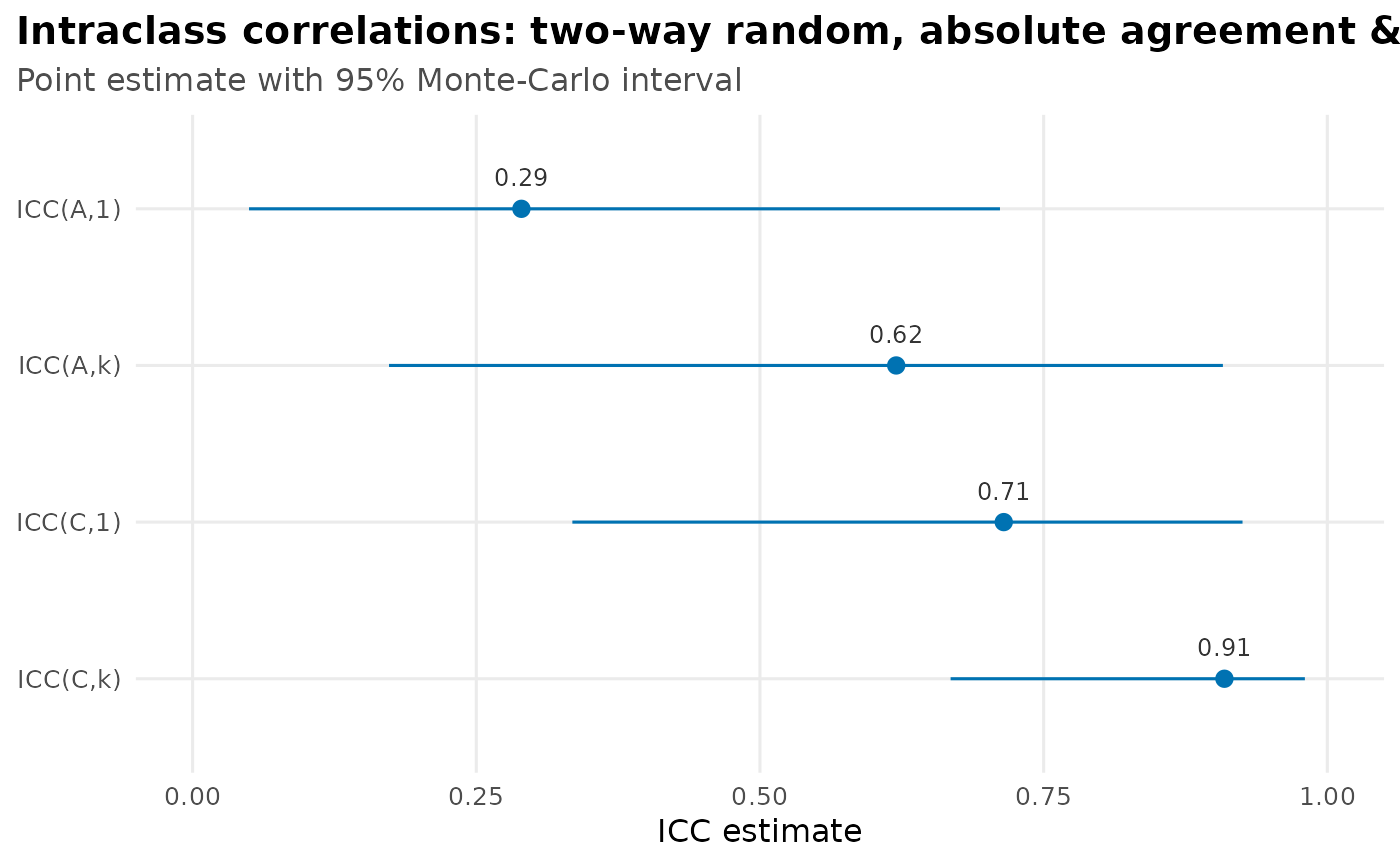ggplot2::autoplot(fit, what = "components") # variance-component decomposition

# `ratings` is the shipped Shrout & Fleiss (1979) worked example: six
# subjects rated by all four raters, in the long layout `icc()` expects --
# one rating per row, with the subject, the rater, and the score in columns.
head(ratings)
#>   subject rater score
#> 1       1     1     9
#> 2       2     1     6
#> 3       3     1     8
#> 4       4     1     7
#> 5       5     1    10
#> 6       6     1     6

icc(ratings, score, subject, rater, seed = 1)
#> ── Intraclass correlation: two-way random, absolute agreement & consistency ────
#> Subjects: 6 | Raters: 4 (random) | Observations: 24 of 24 cells (complete)
#> Engine: glmmTMB (REML) | CI: 95% montecarlo (10000 draws)
#> 
#>   index     estimate   95% CI
#>   Absolute agreement
#>   ICC(A,1)     0.290   [0.050, 0.706]
#>   ICC(A,k)     0.620   [0.175, 0.906]
#>   Consistency
#>   ICC(C,1)     0.715   [0.339, 0.924]
#>   ICC(C,k)     0.909   [0.672, 0.980]
#> 
#> Variance components: subject 2.556, rater 5.244, residual 1.019
#> Shrout & Fleiss equivalent: ICC(A,1) = ICC(2,1), ICC(A,k) = ICC(2,k)