D-studies and within-cell replicates

library(intraclass)

Two things you can do once you have a fitted icc(). The first is to project its reliability to a different number of raters, a decision study. The second, available when each cell holds more than one rating, is to separate the subject-by-rater interaction from pure error (within-cell replicates). This article also shows the autoplot() methods that visualize a fit. (Unfamiliar terms are defined in the Glossary.)

How many raters do I need? A D-study

ICC(*,1) is the reliability of a single rater and ICC(*,k) the reliability of the mean of the k raters you actually used. A decision (D-) study asks a forward-looking question: how reliable would the mean of some other number of raters m be? In generalizability theory the absolute-agreement ICC is the dependability coefficient, and projecting it to m raters is just a change of the averaging divisor,

$$\Phi(m) = \frac{\sigma^2_s}{\sigma^2_s + (\sigma^2_r + \sigma^2_{res}) / m},$$

so d_study() reuses the fit you already have, with no refitting.

fit <- icc(ratings, score, subject, rater, type = "agreement", seed = 1)
proj <- d_study(fit, m = 1:8, seed = 1)
proj
#> # D-study projection: two-way random, absolute agreement
#> Observed raters: 4 | CI: 95% montecarlo (10000 draws)
#>   m  estimate          95% CI
#>   1     0.290  [0.050, 0.706]
#>   2     0.449  [0.096, 0.828]
#>   3     0.550  [0.137, 0.878]
#>   4     0.620  [0.175, 0.906]
#>   5     0.671  [0.210, 0.923]
#>   6     0.710  [0.241, 0.935]
#>   7     0.741  [0.271, 0.944]
#>   8     0.765  [0.298, 0.950]

Reliability climbs with more raters, but with diminishing returns. The projection is anchored to what you observed: at m = 4, the number of raters in ratings, Φ(m) is exactly the ICC(A,k) you would get from icc() directly.

The projection has its own interval settings: conf_level, mc_samples and seed. Each defaults to the fit’s own whenever the fit carries them, which a default Monte-Carlo fit does. Pass any of them to d_study() to override it for this call alone. The seed = 1 above is the fit’s own seed passed explicitly. That is why the m = 4 row reproduces the fit’s ICC(A,k) interval exactly, and not merely its estimate.

tidy() turns the projection into one row per projected point, and glance() summarizes the projection as a whole:

tidy(proj)
#> # A tibble: 8 × 11
#>       m occasions level term     type      estimate std.error conf.low conf.high
#>   <int>     <dbl> <chr> <chr>    <chr>        <dbl>     <dbl>    <dbl>     <dbl>
#> 1     1        NA NA    ICC(A,1) agreement    0.290     0.180   0.0503     0.706
#> 2     2        NA NA    ICC(A,2) agreement    0.449     0.203   0.0959     0.828
#> 3     3        NA NA    ICC(A,3) agreement    0.550     0.205   0.137      0.878
#> 4     4        NA NA    ICC(A,4) agreement    0.620     0.202   0.175      0.906
#> 5     5        NA NA    ICC(A,5) agreement    0.671     0.196   0.210      0.923
#> 6     6        NA NA    ICC(A,6) agreement    0.710     0.189   0.241      0.935
#> 7     7        NA NA    ICC(A,7) agreement    0.741     0.182   0.271      0.944
#> 8     8        NA NA    ICC(A,8) agreement    0.765     0.176   0.298      0.950
#> # ℹ 2 more variables: conf.level <dbl>, method <chr>

glance(proj)
#> # A tibble: 1 × 9
#>     n_m m_min m_max type      raters k_observed conf.level method     mc_samples
#>   <int> <int> <int> <chr>     <chr>       <int>      <dbl> <chr>           <int>
#> 1     8     1     8 agreement random          4       0.95 montecarlo      10000

The one column here that tidy() on the fit does not also give you is m, the rater-count column. That column is the whole point of a D-study: the same coefficient, indexed by the rater count it is projected to. glance() describes the projection rather than the model, reporting the swept range (n_m, m_min, m_max) alongside the design and the interval settings.

We fit with type = "agreement" here because the dependability coefficient above is the absolute-agreement projection. A default icc() reports both agreement and consistency, and d_study() then projects one curve per error definition, told apart by the type column. That is handy when you want both, but for this walkthrough one curve keeps the picture clear.

Read as a curve, this is the classic “how many raters?” picture. Plot it with autoplot(), which needs ggplot2:

library(ggplot2)
autoplot(d_study(fit, m = 1:12))

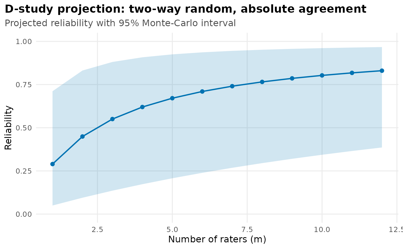
There is also a plot() method, for the console habit of drawing a picture as a side effect. plot() on a projection prints the very same ggplot that autoplot() builds from it, then returns the projection invisibly. We show the call rather than run it, since running it would render another reliability curve just like the one above:

plot(proj)

One projected value, without a projection object

When you want a single projected rater count rather than a whole curve, icc() will report it inline. unit takes the keywords "single" and "average", which give the ICC(*,1) and ICC(*,k) you always get. Alongside them it also takes any number m >= 1:

icc(ratings, score, subject, rater,
  type = "agreement", unit = c("single", "average", 6), seed = 1
)
#> ── Intraclass correlation: two-way random, absolute agreement ──────────────────
#> Subjects: 6 | Raters: 4 (random) | Observations: 24 of 24 cells (complete)
#> Engine: glmmTMB (REML) | CI: 95% montecarlo (10000 draws)
#> 
#>   index     estimate   95% CI
#>   ICC(A,1)     0.290   [0.050, 0.706]
#>   ICC(A,k)     0.620   [0.175, 0.906]
#>   ICC(A,6)     0.710   [0.241, 0.935]
#> 
#> Variance components: subject 2.556, rater 5.244, residual 1.019
#> Shrout & Fleiss equivalent: ICC(A,1) = ICC(2,1), ICC(A,k) = ICC(2,k)

The extra row is labeled ICC(A,6), and it is the same quantity d_study() projects: the m = 6 row of proj above carries the same estimate. The interval matches too, but only because both calls pass the same seed. The interval is Monte-Carlo, so two unseeded runs of the same projection agree on the estimate and differ in the last digits of the endpoints. Which one you reach for is a matter of shape, not of arithmetic: unit adds a row to a coefficient table, while d_study() returns a projection object you can tidy(), glance() and plot.

Fixed raters cannot be projected to absolute agreement. The rater term for fixed raters is the variance of exactly the raters you observed. There is no wider pool for a hypothetical sixth rater to be drawn from, so icc() refuses rather than returning a number:

icc(ratings, score, subject, rater,
  type = "agreement", raters = "fixed", unit = c("single", "average", 6),
  seed = 1
)
#> Error in `icc()`:
#> ! Projecting absolute agreement to a different number of raters is not
#>   defined for "fixed" raters.
#> ℹ With fixed raters the rater term is the finite-population variance of exactly
#>   the raters you observed, so there is no 'average of m freshly sampled raters'
#>   to project to.
#> ℹ Use `raters = "random"` to project absolute agreement, or `type =
#>   "consistency"` for a fixed-rater D-study.

Consistency has no such problem, because the rater term drops out of it. That is why the two remedies the message names are to project with raters = "random", or to ask for a fixed-rater type = "consistency" projection instead. The refusal is raised only when absolute agreement is all you asked for. A default icc() call reports both error definitions, and there the consistency projection is kept and you are told the agreement one was dropped.

Projection is extrapolation. The rater variance $\sigma^2_r$ is estimated from only as many raters as you observed, so projecting far beyond that design leans hard on that estimate. The Monte-Carlo interval widens honestly to reflect this, rather than pretending to a precision it lacks. And projecting absolute agreement is refused for fixed raters, where there is no wider rater universe to generalize to (use raters = "random"). The D-study also works on a multilevel fit, projecting the rater count at each level.

Within-cell replicates: interaction vs. pure error

So far every subject-by-rater cell holds a single rating. When each rater rates each subject more than once, a design with within-cell replicates, you can separate two things that a single rating confounds. The first is the subject-by-rater interaction: does a rater systematically score a particular subject high or low, a stable disagreement? The second is pure error, meaning how much a rater’s repeat ratings of the same subject wobble. icc() detects the replicates and fits the interaction model automatically:

set.seed(2025)
ns <- 20
nr <- 4
no <- 3
grid <- expand.grid(subject = seq_len(ns), rater = seq_len(nr), occ = seq_len(no))
subj <- rnorm(ns, sd = 1.1)[grid$subject]
rater <- rnorm(nr, sd = 0.8)[grid$rater]
sr <- rnorm(ns * nr, sd = 0.6)[(grid$rater - 1) * ns + grid$subject]
reps <- data.frame(
  subject = factor(grid$subject),
  rater = factor(grid$rater),
  score = 10 + subj + rater + sr + rnorm(nrow(grid), sd = 0.7)
)

icc(reps, score, subject, rater, type = "agreement", occasions = c("single", "average"))
#> ── Intraclass correlation: two-way random, absolute agreement ──────────────────
#> Subjects: 20 | Raters: 4 (random) | 80 cells x 3 replicates (complete)
#> Engine: glmmTMB (REML) | CI: 95% montecarlo (10000 draws)
#> 
#>   index     occasions estimate   95% CI
#>   ICC(A,1)          1    0.263   [0.083, 0.489]
#>   ICC(A,1)          3    0.300   [0.088, 0.562]
#>   ICC(A,k)          1    0.588   [0.265, 0.793]
#>   ICC(A,k)          3    0.631   [0.279, 0.837]
#> 
#> Variance components: subject 0.631, rater 0.901, subject:rater 0.428, residual 0.443
#> Shrout & Fleiss equivalent: ICC(A,1) = ICC(2,1), ICC(A,k) = ICC(2,k)

The variance-components line now shows subject:rater (the interaction) and residual (pure error) as separate terms. The single-occasion rows, whose occasions column reads 1, are the ordinary ICCs, since a single rating’s error still includes the interaction. But they are now fit correctly, rather than folding the interaction into the residual. The occasion-averaged rows, whose occasions column reads 3 here, divide pure error by three occasions per rater. ICC(A,1) is then the reliability of one rater’s mean of three ratings. ICC(A,k) is the reliability of a mean over all four raters, each at that same three. That 3 is the fitted per-cell replicate count. Averaging cuts pure error but not the interaction, so those coefficients are higher.

Within-cell replicates extend beyond this balanced two-way random example: fixed raters (balanced), multilevel designs (crossed Design 1 and nested Design 2, balanced), and ragged replicates at a single occasion are all supported. What remains open is the occasion-averaged coefficient on ragged replicates, where unequal per-cell counts leave no single effective-occasion divisor with a validated oracle. The compound fixed-by-ragged and multilevel-by-ragged corners are open too.

How many occasions do I need? A D-study on the occasion facet

Just as d_study(m = ...) projects the number of raters, d_study(n_o = ...) projects the number of occasions off a replicate fit. It holds the raters fixed and asks “how reliable would each rater’s mean of n_o ratings be?”. Supply exactly one axis per call (m or n_o).

fit_rep <- icc(reps, score, subject, rater, type = "agreement", occasions = "average")
d_study(fit_rep, n_o = 1:6)
#> # D-study projection: two-way random, absolute agreement
#> Held raters: 4 (average) | projecting occasions | CI: 95% montecarlo (10000 draws)
#>   n_o  m  estimate          95% CI
#>     1  4     0.588  [0.265, 0.791]
#>     2  4     0.620  [0.277, 0.824]
#>     3  4     0.631  [0.280, 0.835]
#>     4  4     0.637  [0.282, 0.841]
#>     5  4     0.641  [0.283, 0.845]
#>     6  4     0.643  [0.284, 0.847]

Notice the curve flattens. Averaging more occasions only cancels pure error (residual). It never touches the rater or subject:rater variance. So the occasion curve climbs to a ceiling below 1, rather than approaching 1 the way a rater projection does. That ceiling is the reliability you would reach with perfectly repeatable ratings but the same raters. Read it as “how much does re-rating help?”, which saturates.

Because occasions are a random facet however the raters are treated, the occasion projection is defined even where a rater projection is not: fixed-rater absolute agreement projects on the occasion axis. It is only the rater axis that is undefined for fixed absolute agreement, having no “freshly sampled rater” to add. On a multilevel replicate fit the subject-level curve rises with n_o while the cluster-level curve is flat. The cluster-level error set has no pure-error term, so occasions cannot change it, and d_study() says so with a note.

Visualizing a fit

Every icc() fit carries an autoplot() method (with a plot() wrapper), so you can see the coefficients and the variance components behind them without building a plot by hand. Both read straight off the fitted object, so the picture can never disagree with the printed table. They need ggplot2, an optional dependency.

The default, what = "coefficients", is a forest plot: each ICC index as a point estimate with its Monte-Carlo interval. Reusing the two-way ratings fit from the D-study section above:

library(ggplot2)
autoplot(fit) # `fit <- icc(ratings, score, subject, rater, type = "agreement", seed = 1)`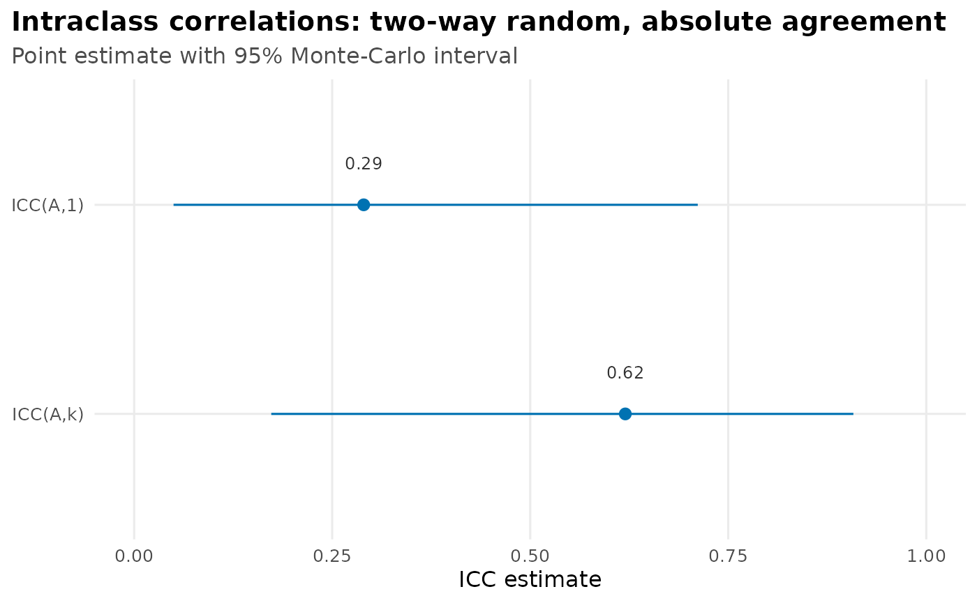

what = "components" shows the other half of the story: the estimated variance components the ratio is built from. It makes plain why absolute agreement is so much lower than the averaged coefficient on ratings. The rater component is large, and only absolute agreement counts between-rater differences as error:

autoplot(fit, what = "components")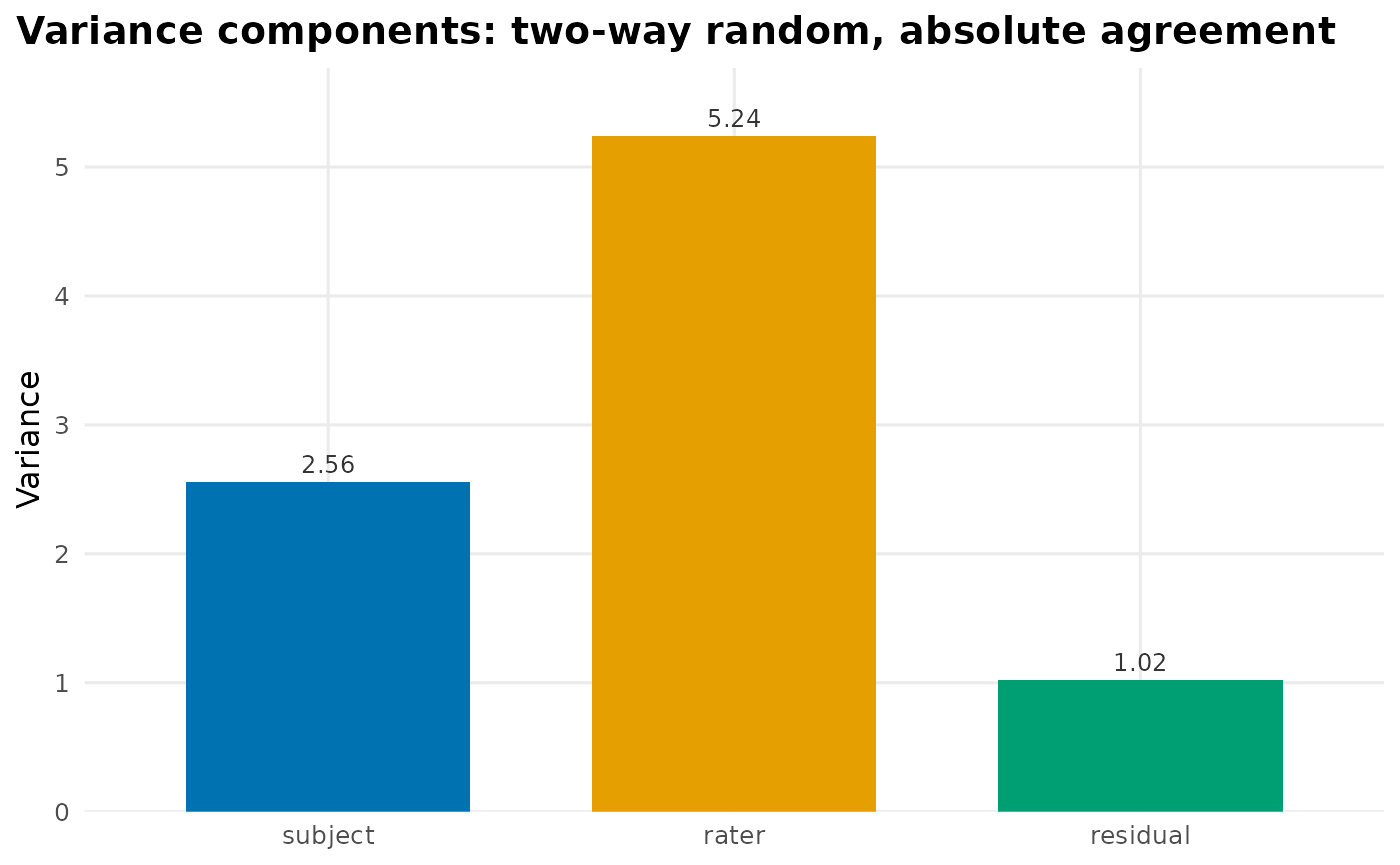

For a multilevel fit the forest plot facets by level. See Multilevel designs for that example.