
Multilevel designs: subject and cluster level
Source:vignettes/multilevel-designs.Rmd
multilevel-designs.RmdThe Getting started and Choosing an ICC articles treat the subject as the object of measurement. But subjects are often nested in higher-level clusters, such as pupils in classrooms or patients in clinics. Then “reliability” splits in two: how well raters tell subjects apart, and how well they tell clusters apart. The second is the cluster-level ICC, where the subject level is reliability within a cluster, and the cluster level is reliability of cluster means. Those are different questions with different answers. Reporting one when you needed the other can be badly misleading. Ignoring the nesting gives a conflated ICC, the single-level ICC that ignores clustering, which is biased for both questions.
This article covers the multilevel ICC family of ten Hove, Jorgensen & van der Ark (2022). Its coefficients are ratios of variance components, each a share of the total variation traced to one source. The family spans crossed and nested layouts, complete and incomplete data, and fixed raters, where the observed raters are the whole population of interest. It ends with the multilevel D-study, which projects the fitted variance components to other rater or occasion counts. Any unfamiliar term is defined in the Glossary.
Subject level vs. cluster level
When subjects are nested in clusters, two reliabilities are defined:
- Subject level (within-cluster): how reliably do raters distinguish subjects within a cluster?
- Cluster level (between-cluster): how reliably do raters distinguish cluster means?
Ignoring the nesting conflates these and biases both (ten
Hove, Jorgensen & van der Ark, 2022). Passing a cluster
column to icc() fits the multilevel model and reports each
level separately.
Consider pupils nested in classrooms, each pupil rated by the same
panel of raters. The shipped school data are a simulated
design of this kind: 16 classrooms, 5 pupils in each, and the same 4
raters scoring every pupil. The simulation puts substantial signal at
the classroom level and modest differences within a classroom (see
?school for how it is built):
str(school)
#> 'data.frame':    320 obs. of  4 variables:
#>  $ classroom: Factor w/ 16 levels "1","2","3","4",..: 1 1 1 1 1 2 2 2 2 2 ...
#>  $ pupil    : Factor w/ 80 levels "1_1","1_2","1_3",..: 1 2 3 4 5 6 7 8 9 10 ...
#>  $ rater    : Factor w/ 4 levels "1","2","3","4": 1 1 1 1 1 1 1 1 1 1 ...
#>  $ score    : num  10.5 10.1 10 11.7 9 ...
icc(school, score, subject = pupil, rater = rater, cluster = classroom, type = "agreement", seed = 1)
#> ℹ Treating raters with the same label in different clusters as the same raters
#>   (crossed with clusters, Design 1).
#> ℹ If each cluster has its own raters, give them cluster-unique labels or pass
#>   `design = "nested_in_clusters"`.
#> ── Intraclass correlation: multilevel two-way random, absolute agreement ───────
#> Subjects: 80 in 16 clusters | Raters: 4 (random) | Observations: 320 (complete)
#> Engine: glmmTMB (REML) | CI: 95% montecarlo (10000 draws)
#>
#>   level      index     estimate   95% CI
#>   subject    ICC(A,1)     0.431   [0.251, 0.562]
#>   subject    ICC(A,k)     0.751   [0.573, 0.837]
#>   cluster    ICC(A,1)     0.880   [0.000, 0.973]
#>   cluster    ICC(A,k)     0.967   [0.000, 0.993]
#>
#> Variance components: cluster 0.998, subject 0.461, rater 0.136, cluster:rater 0.000, residual 0.473
#>
#> This message is displayed once per session.
Both levels come back in one call. Here the
cluster-level ICC is the higher of the two. Raters
agree more about which classrooms score high than about which
pupils within a classroom do. That is exactly the pattern you
would expect when most of the true variation lives between classrooms.
Which number you report depends on the decision you will make. A
classroom-level intervention cares about the cluster-level reliability,
a pupil-level one about the subject level. Request just one with
level = "subject" or level = "cluster".
How much does ignoring the nesting cost? The conflated ICC
What would you have reported if you had ignored the
classrooms and run an ordinary single-level ICC? That number is ten Hove
et al.’s Equation 14. It folds the between-classroom and
within-classroom variation together into one “true score”, and is biased
for both questions above. icc() can
compute this conflated ICC as a diagnostic contrast
with level = "conflated". So you can see the distortion
directly rather than take it on faith:
icc(school, score,
  subject = pupil, rater = rater, cluster = classroom,
  type = "agreement", level = c("subject", "cluster", "conflated"), seed = 1
)
#> ── Intraclass correlation: multilevel two-way random, absolute agreement ───────
#> Subjects: 80 in 16 clusters | Raters: 4 (random) | Observations: 320 (complete)
#> Engine: glmmTMB (REML) | CI: 95% montecarlo (10000 draws)
#>
#>   level      index     estimate   95% CI
#>   subject    ICC(A,1)     0.431   [0.251, 0.562]
#>   subject    ICC(A,k)     0.751   [0.573, 0.837]
#>   cluster    ICC(A,1)     0.880   [0.000, 0.973]
#>   cluster    ICC(A,k)     0.967   [0.000, 0.993]
#>   conflated  ICC(A,1)     0.705   [0.000, 0.808]
#>   conflated  ICC(A,k)     0.905   [0.000, 0.944]
#>
#> Variance components: cluster 0.998, subject 0.461, rater 0.136, cluster:rater 0.000, residual 0.473
#> Diagnostic contrast: the 'conflated' level ignores the cluster structure
#> (ten Hove et al. 2022, Eq. 14). It shows the bias from a single-level
#> analysis and is NOT a recommended coefficient. Report the subject level,
#> the cluster level, or both.
The conflated value lands between the two correct levels and matches
neither: it over- or under-states the reliability of any real decision.
It is printed with a warning label and is never a
coefficient to report. It exists only to quantify the cost of ignoring
the structure. It is the flat two-way ICC read off the fit, the design
where each rater is tracked across the subjects they score. So it comes
in two forms. One is absolute agreement, where raters give the same
score. The other is consistency,
where raters agree apart from a constant offset per rater. A default
level = "conflated" call reports both. It needs a crossed,
random-rater design with raters that bridge the clusters, and works on
complete or incomplete data.
When raters are nested
The classroom example above has every rater rate every pupil in every
classroom. So raters are crossed with clusters: ten
Hove et al.’s Design 1, where one panel of raters spans every cluster.
Two other layouts are common, and icc() infers
which one you have from the crossing pattern. That pattern is
which raters appear in which clusters, and which pupils each of them
rates. The design argument overrides that inference, and
there are two reasons to reach for it. The first is when the rater
labels do not mean what the pattern implies (Declaring
the design below). The second is when missing cells leave the
pattern genuinely ambiguous (Incomplete (ragged)
multilevel designs). The two nested layouts are:
-
Raters nested in clusters (Design 2): each
classroom has its own panel of raters. Under Design 2 there is
then no between-cluster reliability to report. A cluster-level ICC needs
the same raters spanning clusters, so
icc()returns the subject level only. -
Raters nested in subjects (Design 3): each pupil is
rated by their own raters. Now systematic rater differences
cannot be separated from residual error at all. So this is a multilevel
one-way design: it reports agreement-only
ICC(1)/ICC(k), the clustered analogue ofmodel = "oneway".
Take the same classrooms but give each one its own raters (Design 2):
school_d2 <- school
school_d2$rater <- factor(paste(school_d2$classroom, school_d2$rater, sep = "_"))
icc(school_d2, score, subject = pupil, rater = rater, cluster = classroom, type = "agreement", seed = 1)
#> ── Intraclass correlation: multilevel (raters nested in clusters) two-way random
#> Subjects: 80 in 16 clusters | Raters: 64 (random) | Observations: 320 (complete)
#> Engine: glmmTMB (REML) | CI: 95% montecarlo (10000 draws)
#>
#>   level      index     estimate   95% CI
#>   subject    ICC(A,1)     0.429   [0.310, 0.549]
#>   subject    ICC(A,k)     0.751   [0.643, 0.829]
#>
#> Variance components: cluster 0.966, subject 0.458, rater:cluster 0.128, residual 0.481
The header now reads raters nested in clusters and only the subject level comes back. If instead each pupil has their own raters, the design is a multilevel one-way (Design 3):
school_d3 <- school
school_d3$rater <- factor(paste(school_d3$pupil, school_d3$rater, sep = "_"))
icc(school_d3, score, subject = pupil, rater = rater, cluster = classroom, type = "agreement", seed = 1)
#> ── Intraclass correlation: multilevel (raters nested in subjects) absolute agree
#> Subjects: 80 in 16 clusters | Raters: 320 | Observations: 320 (complete)
#> Engine: glmmTMB (REML) | CI: 95% montecarlo (10000 draws)
#>
#>   level      index     estimate   95% CI
#>   subject    ICC(1)       0.412   [0.290, 0.543]
#>   subject    ICC(k)       0.737   [0.620, 0.826]
#>
#> Variance components: cluster 0.998, subject 0.426, residual 0.609 (rater confounded)
Here the coefficients are labeled ICC(1) /
ICC(k) and type no longer applies. With each
pupil’s raters unique, there is no rater main effect to keep in or drop
from the error term. A layout that is neither cleanly crossed nor
cleanly nested raises an informative error rather than guessing at a
model. One such layout has some raters shared across clusters and some
not.
Declaring the design when the labels are ambiguous
Both relabellings above worked by rewriting the rater column.
Inference reads that column and can only be as good as the labels in it.
The school table as built numbers its raters 1–4 inside
every classroom. Nothing in the data says whether “rater 1” in
classroom 3 is the same person as “rater 1” in classroom 7. Left to
itself icc() reads the reused labels as one panel rating
everywhere, which is Design 1, and says so rather than deciding quietly.
If the numbering is instead classroom-relative, say so with
design:
icc(school, score,
  subject = pupil, rater = rater, cluster = classroom,
  type = "agreement", design = "nested_in_clusters", seed = 1
)
#> ── Intraclass correlation: multilevel (raters nested in clusters) two-way random
#> Subjects: 80 in 16 clusters | Raters: 4 (random) | Observations: 320 (complete)
#> Engine: glmmTMB (REML) | CI: 95% montecarlo (10000 draws)
#>
#>   level      index     estimate   95% CI
#>   subject    ICC(A,1)     0.429   [0.310, 0.549]
#>   subject    ICC(A,k)     0.751   [0.643, 0.829]
#>
#> Variance components: cluster 0.966, subject 0.458, rater:cluster 0.128, residual 0.481
The header now reads raters nested in clusters and the
cluster level is gone. A single rater:cluster component
replaces the two rater terms the crossed fit printed (rater
and cluster:rater). If the numbering is
pupil-relative, meaning each pupil’s own four raters numbered
from one, the same table is Design 3:
icc(school, score,
  subject = pupil, rater = rater, cluster = classroom,
  type = "agreement", design = "nested_in_subjects", seed = 1
)
#> ── Intraclass correlation: multilevel (raters nested in subjects) absolute agree
#> Subjects: 80 in 16 clusters | Raters: 4 | Observations: 320 (complete)
#> Engine: glmmTMB (REML) | CI: 95% montecarlo (10000 draws)
#>
#>   level      index     estimate   95% CI
#>   subject    ICC(1)       0.412   [0.290, 0.543]
#>   subject    ICC(k)       0.737   [0.620, 0.826]
#>
#> Variance components: cluster 0.998, subject 0.426, residual 0.609 (rater confounded)
Now there is no rater term at all. The components line reports the
residual as (rater confounded). The coefficients are the
agreement-only ICC(1) / ICC(k) of the
multilevel one-way design.
One table, three readings, and the data cannot tell you which is
right: only you know what the labels mean. So icc()
announces the crossed reading in a message rather than assuming it
quietly. The message prints once per session, so in this article it
appeared back at the first classroom fit. What separates the three
readings is mostly structure rather than the subject-level number.
Moving to Design 2 barely moves the subject coefficients
(ICC(A,1) 0.431 crossed against 0.429 here), but takes the
cluster level away. Moving to Design 3 takes the rater term with it and
renames the coefficients.
Declaring a design is still bounded by the data:
design = "crossed" on raters that do not bridge clusters is
refused, for either error definition. What a declaration can do
unchecked is choose among the readings the data does admit, the choice
made twice above. So declare a design only when you know the labelling.
Where the labels are already unique per rater, as in the two relabelled
tables earlier, inference has everything it needs. Passing the matching
design explicitly then returns the very same fit.
Incomplete (ragged) multilevel designs
The Choosing an ICC
article works a connected
incomplete design, one where raters and subjects form one linked web.
Just as in that single-level case, the crossed design
(Design 1) does not need every pupil rated by every rater. The mixed
model estimates the variance components from whatever cells are present,
so a ragged classroom design is handled directly. The shipped
school_incomplete data are the school data
with a fifth of the ratings dropped at random:
At the subject level both agreement and consistency
come back. This matches the single-level incomplete case.
ICC(*,k) averages over the effective
number of ratings (k_eff): the harmonic mean of the
per-subject rating counts, an average that leans toward the smaller
values. It is below the full panel size of 4:
icc(school_incomplete, score, subject = pupil, rater = rater, cluster = classroom,
  type = "agreement", level = "subject", seed = 1)
#> ── Intraclass correlation: multilevel two-way random, absolute agreement ───────
#> Subjects: 80 in 16 clusters | Raters: 4 (random) | Observations: 256 (incomplete)
#> Engine: glmmTMB (REML) | CI: 95% montecarlo (10000 draws)
#>
#>   level      index     estimate   95% CI
#>   subject    ICC(A,1)     0.413   [0.233, 0.557]
#>   subject    ICC(A,k)     0.673   [0.470, 0.786]
#>
#> ICC(*,k) projects to an effective 2.93 raters (harmonic mean of ratings/subject).
#> Variance components: cluster 1.026, subject 0.409, rater 0.125, cluster:rater 0.000, residual 0.457
The header now reads incomplete, and the report names the
effective k so the divisor is never a black box.
At the cluster level, both ICC(c,1) and
the averaged ICC(c,k) come back on ragged
data. The averaged coefficient divides the cluster error by its own
effective rater count, the raters behind each classroom’s observed mean.
That count is reported as k_c_eff (the inverse-Simpson
harmonic mean), and it is not the same as the per-pupil
k_eff:
icc(school_incomplete, score, subject = pupil, rater = rater, cluster = classroom,
  level = "cluster", type = c("agreement", "consistency"),
  unit = c("single", "average"), seed = 1)
#> ── Intraclass correlation: multilevel two-way random, absolute agreement & consi
#> Subjects: 80 in 16 clusters | Raters: 4 (random) | Observations: 256 (incomplete)
#> Engine: glmmTMB (REML) | CI: 95% montecarlo (10000 draws)
#>
#>   level      index     estimate   95% CI
#>   Absolute agreement
#>   cluster    ICC(A,1)     0.892   [0.000, 0.976]
#>   cluster    ICC(A,k)     0.970   [0.000, 0.994]
#>   Consistency
#>   cluster    ICC(C,1)     1.000   [0.000, 1.000]
#>   cluster    ICC(C,k)     1.000   [0.000, 1.000]
#>
#> Cluster ICC(c,k) averages over an effective 3.87 raters (inverse-Simpson k_c^eff).
#> Variance components: cluster 1.026, subject 0.409, rater 0.125, cluster:rater 0.000, residual 0.457
One subtlety worth knowing. On ragged data, systematic rater
differences no longer cancel perfectly from a comparison of
observed cluster means. They cancel only when every cluster has the same
rater weighting. If you are ranking clusters by their observed means,
prefer the agreement ICC(c,k), whose error
term accounts for that. The consistency ICC(c,k) measures
cluster×rater disagreement only. This averaged cluster coefficient on
ragged data ships for every random-rater engine, the software that does the
fitting: glmmTMB, lme4, and the Bayesian
brms engine. The brms engine applies the same
k_c_eff divisor to its posterior draws.
One thing is still deliberately fenced off, with a clear error rather
than a silently wrong number. Missing cells can make the crossing
pattern ambiguous. Some raters happen to appear in only
one classroom, so the design could be read as crossed or
nested. There icc() does not guess. You resolve it by
declaring design = "crossed", which is validated against
the data, or the abort points you at the nested reading.
Fixed raters in a multilevel design
The multilevel examples so far treat raters as a random
sample, the recommended default. A random sample generalizes beyond
the raters you happened to use. When the observed raters are
the entire population of interest (a fixed panel of examiners, say),
pass raters = "fixed". As in the single-level case, the
rater main effect is then the finite-population
variance of these raters: the spread of just the observed
raters. That is McGraw & Wong’s Case 3A, not a random-sample
variance. On a balanced crossed design both levels come back:
icc(school, score, subject = pupil, rater = rater, cluster = classroom,
  type = "agreement", raters = "fixed")
#> Warning: Modeling raters as fixed restricts inference to exactly these raters. You
#> cannot generalize to other raters.
#> ℹ For interrater reliability, the two-way random model (`raters = "random"`) is
#>   the recommended default (ten Hove et al. 2024; McGraw & Wong 1996, Case 2).
#> ℹ Use "fixed" only when these are the entire population of raters you will ever
#>   use.
#> ── Intraclass correlation: multilevel two-way mixed, absolute agreement ────────
#> Subjects: 80 in 16 clusters | Raters: 4 (fixed) | Observations: 320 (complete)
#> Engine: glmmTMB (REML) | CI: 95% montecarlo (10000 draws)
#>
#>   level      index     estimate   95% CI
#>   subject    ICC(A,1)     0.431   [0.318, 0.549]
#>   subject    ICC(A,k)     0.751   [0.651, 0.830]
#>   cluster    ICC(A,1)     0.880   [0.000, 0.944]
#>   cluster    ICC(A,k)     0.967   [0.000, 0.985]
#>
#> Variance components: cluster 0.998, subject 0.461, rater 0.136, cluster:rater 0.000, residual 0.473
On this balanced design the fixed-rater coefficients match the random-rater ones at both levels. Consistency never uses the rater term, so it is identical either way. Absolute agreement coincides because the finite-population rater variance equals the random-sample estimate when the design is balanced. At the cluster level the between-rater disagreement in cluster means is that same finite-population term plus the cluster-by-rater interaction. The subject level genuinely diverges from random on incomplete data, where the rater variance is estimated from unequal cell counts. And the crossed (Design 1) fixed-rater multilevel design is supported on ragged data too, at the subject level, exactly as the single-level incomplete case above.
Multilevel support now covers random raters on the
crossed design (Design 1), complete or incomplete, at
the subject level and the cluster level. That covers both
ICC(c,1) and the averaged ICC(c,k), across all
three engines (glmmTMB, lme4,
brms). It also covers the nested designs (Designs 2 and 3,
subject level), complete or incomplete. The
structural-equation lavaan engine joins them on the crossed
design for complete, balanced data with equal cluster
sizes. A two-level SEM estimates the same five-component decomposition
and reports both levels. See the engines
vignette for how its estimator differs from the mixed-model one at
small cluster counts. Fixed raters are supported at the
subject level on the crossed design (complete and
incomplete). They are also supported at the cluster
level on the crossed design (complete data), and, on complete data, the
nested Design 2. What remains open is incomplete fixed-rater
cluster-level estimation. Design 3 reports no fixed-rater or
cluster-level coefficient by construction. With raters nested in
subjects there is no separable rater effect to fix, and no
crossed-cluster structure to support a cluster mean.
How many raters? A multilevel D-study
The D-study works on a
multilevel fit too. It projects the number of raters at
each level. So you can ask “how many raters would make the
cluster-level score reliable?” separately from the subject
level. It returns one curve per level (note the level
column), and autoplot() facets them:
d_study(
  icc(school, score, subject = pupil, rater = rater, cluster = classroom, type = "agreement", seed = 1),
  m = c(1, 2, 4, 8)
)
#> # D-study projection: multilevel two-way random, absolute agreement
#> Observed raters: 4 | CI: 95% montecarlo (10000 draws)
#>     level  m  estimate          95% CI
#>   subject  1     0.431  [0.251, 0.562]
#>   subject  2     0.602  [0.402, 0.720]
#>   subject  4     0.751  [0.573, 0.837]
#>   subject  8     0.858  [0.729, 0.911]
#>   cluster  1     0.880  [0.000, 0.973]
#>   cluster  2     0.936  [0.000, 0.986]
#>   cluster  4     0.967  [0.000, 0.993]
#>   cluster  8     0.983  [0.000, 0.997]
Only the rater count is projected. The cluster-level coefficient does not average over subjects (ten Hove et al. 2022, Eq. 13). So “how many subjects per cluster?” is a sample-size question, about the precision of your variance-component estimates. It is not a reliability projection.
Visualizing the levels
The autoplot() forest plot facets a
multilevel fit by level, so the subject-level and
cluster-level coefficients line up for comparison. See the D-studies
article for the single-level version. Below is the same
school fit from above, whose cluster level was the higher
of the two:
library(ggplot2)
autoplot(icc(school, score, subject = pupil, rater = rater, cluster = classroom,
  type = "agreement", seed = 1))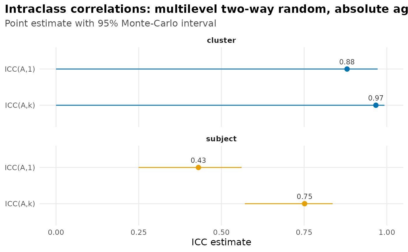
Or let the package choose the level
The multilevel fifth choice, subject level against cluster
level, is part of the choose_icc() decision helper too. The
Choosing an ICC guide walks
the other four axes. Pass the design and it hands back the coefficient
or coefficients to report and the exact icc() call, without
fitting anything:
choose_icc(model = "twoway", multilevel = TRUE, level = "cluster",
  type = "consistency", unit = "single", raters = "random")
#> ── Recommended ICC ─────────────────────────────────────────────────────────────
#> Design: multilevel, two-way random, consistency
#>
#> Recommendation:
#>   cluster: ICC(C,1)
#>
#> Why:
#>   - Crossed (two-way): each rater is tracked across the subjects they score.
#>   - Consistency: only the rank order must match. A constant per-rater offset is forgiven.
#>   - Single rater: you will act on one rater's score.
#>   - Random raters: a sample you generalize beyond, to the rater universe they were drawn from.
#>   - Cluster level: reliability of the cluster mean.
#>
#> Run this on your data:
#>   icc(data, score, subject, rater, cluster, type = "consistency", unit = "single", level = "cluster")
#>
#> Notes:
#>   - Complete vs. incomplete is automatic: icc() uses whatever ratings are present and projects ICC(*,k) to the effective number of ratings (k_eff). The design must stay connected, or icc() fails loudly.
#>   - See vignette("multilevel-designs") for a worked multilevel example.
The helper is generated from the same estimand machinery as
icc(), the estimand being the true quantity you are trying
to estimate. So the emitted call cannot drift from what
icc() actually computes. In an interactive
session you can omit the deciding answers. choose_icc()
will then ask the outstanding questions one at a time, then resolve.