
![[Experimental]](figures/lifecycle-experimental.svg)
Projects the reliability of a fitted icc() to the mean of m raters, for
any m. It reuses the fit's variance components, each a share of the total
variation traced to one source. This is a generalizability-theory decision
study (D-study), which projects the fitted variance components to other
rater or
occasion
counts. It answers "how reliable would the mean of m raters be?"
and, read as a curve, "how many raters do I need?". The point estimate and
its interval reuse the fit stored on x, and no model is refit. The
interval is boundary-aware, since an estimate can land exactly at zero. The
band follows the fit's ci_method. A Monte-Carlo fit has an interval
built by drawing parameter values from the fitted model's uncertainty. It
reprojects one draw from the parameter covariance across every m. A bootstrap fit, which refits the
model on simulated data many times, reprojects its stored resamples. So on
a bootstrap fit, at m = the observed rater count the band matches the
fitted ICC(*,k) interval exactly.
Usage
autoplot.intraclass_dstudy(object, ...)

# S3 method for class 'intraclass_dstudy'
plot(x, ...)

d_study(
  x,
  m = NULL,
  n_o = NULL,
  conf_level = NULL,
  mc_samples = NULL,
  seed = NULL
)

# S3 method for class 'intraclass_dstudy'
format(x, ...)

# S3 method for class 'intraclass_dstudy'
print(x, ...)

# S3 method for class 'intraclass_dstudy'
tidy(x, ...)

# S3 method for class 'intraclass_dstudy'
glance(x, ...)
Arguments
- object
An
intraclass_dstudyobject (theautoplot()/plot()argument).- ...
Unused. Present so the method signature matches the generic.
- x
An
intraclass_iccobject returned byicc().- m
Numeric vector of rater counts to project to (each \(\ge 1\)). Defaults to
1:(2 * n_raters), a curve from one rater to twice the observed count. Mutually exclusive withn_o.- n_o
Numeric vector of occasion (within-cell replicate) counts to project to (each \(\ge 1\)), holding raters at the observed count. This is a D-study on the occasion facet of a within-cell replicate fit. Mutually exclusive with
m, and supplying both aborts.NULL(the default) projects the rater countminstead.- conf_level, mc_samples, seed
Interval settings. Each defaults to the value stored on
x, so a seeded fit yields a reproducible projection. Override to change the confidence level, the number of Monte-Carlo draws, or the seed.
Value
d_study() returns an intraclass_dstudy object: a tibble with one
row per projected point. Its columns are m, index (e.g. "ICC(A,3)"),
type, estimate, std.error, conf.low, and conf.high, and it
carries the design and interval settings as attributes. tidy() names that
coefficient column term, following the broom glossary. The object keeps
index. If the fitted intraclass_icc reports both error definitions (the
default), d_study() projects one reliability curve per definition,
distinguished by the type column. A single-type fit projects a single
curve. A multilevel projection gains a level column (one curve per
level), and a replicate projection an occasions column, each where it
applies. tidy() carries both columns on every projection, NA where the
fit does not define them. Read the projection with tidy(): the object's
own layout is internal, and only the tidied columns are a stable contract.
The methods documented on this page return the objects below.
tidy.intraclass_dstudy(): a tibble with one row per projected point. Its columns, in this order, arem,occasions,level,term,type,estimate,std.error,conf.low,conf.high,conf.level,method.termis the projected ICC index, named for the broom glossary. Every column is present on every projection.occasionsreports the per-cell occasion count the row is projected at, which may be non-integer, and which divides pure error, so a row whose error set carries no pure-error term does not move with it. On a rater projection the column takes every distinct occasion value the fit's owntidy()$occasionscolumn carries, and the cluster rows of a multilevel projection take the smallest of those. On an occasion projection every row takes the sweptn_o, cluster rows included, whose curve is flat across it.occasionsisNAoutside a replicate projection.levelisNAoutside a multilevel one, andtypewhere the design defines no error definition.glance.intraclass_dstudy(): a one-row tibble of projection-level summaries. It carries the distinct projected rater countsmand their range, the error definition(s), the rater treatment, the observed rater count, and the interval settings. The rater treatment isNAon a projection of a fit that estimates no separable rater main effect. One such fit ismodel = "oneway", whose raters are interchangeable and carry no facet. The other isdesign = "nested_in_subjects", whose rater effect is confounded into the residual. The count and range are held at the observed rater count when the sweep is over occasions, so they are not a row count.format.intraclass_dstudy(): a character vector holding the printed projection table, one line per element.print.intraclass_dstudy(): theintraclass_dstudyobject invisibly, having emitted that table.autoplot.intraclass_dstudy(): aggplotobject holding the reliability curve, faceted by level for a multilevel projection.plot.intraclass_dstudy(): theintraclass_dstudyobject invisibly, having drawn that curve.
tidy.intraclass_dstudy() and glance.intraclass_dstudy() implement the
tidy() and glance() generics.
Checks on the band
On a glmmTMB or lme4 fit, whatever its ci_method, d_study() reads each
curve's single-rating coefficient from the band's draws. That is the
coefficient at one rater, and at one occasion on a within-cell replicate
fit. Every projected row of the curve comes from the same draws. If the
two limits of that coefficient's interval are exactly equal, d_study()
refuses the band with an intraclass_zero_width_interval error, which is
also an intraclass_singular_fit error. If the limits differ and the lower
limit lies within 1e-12 of 1, d_study() returns the projection with an
intraclass_unresolved_interval warning. Data with almost no residual
variation can give such an interval. At a very large m, a projected row
can print as [1, 1] through rounding. The checks read only the
single-rating interval, so such a row raises neither the error nor the
warning by itself.
Projection is extrapolation
Projecting to an m you did not run is an extrapolation. Its
trustworthiness depends on how well the variance components are pinned
down. The rater variance \(\sigma^2_r\) matters most, since it is
estimated from only as many raters as you observed. With few raters that
estimate is noisy, so the projected interval is honestly wide. The
Monte-Carlo interval widens automatically, recomputing \(\Phi(m)\) on
every draw rather than pretending a single plugged-in value. m is the
number of raters and is normally an integer, though non-integer values are
permitted.
Projection is defined for random raters, under both error definitions.
Those are agreement, where raters give the same score, and consistency,
where raters agree apart from a constant offset per rater. It is also
defined for fixed-rater consistency, fixed meaning the observed raters
are the whole population of interest. In a two-way design each rater is
tracked across the subjects they score. The one-way model, where raters
are not tracked, is
defined too, as a Spearman-Brown projection of ICC(1). Projection is not
defined for fixed-rater absolute agreement. There the rater term is the
finite-population variance, the spread of just the observed raters. So
there is no "average of m freshly sampled raters" to project to.
d_study() aborts in that case (use raters = "random").
Multilevel projections
For a multilevel fit (a cluster column), d_study() projects the rater
count m for each correctly-partitioned level on the object. Those are the
subject and/or cluster level, where the subject level is reliability
within a cluster, and the cluster level is reliability of cluster means. It
returns one reliability curve per
level, and the returned object gains a level column that autoplot()
facets by. tidy() carries that column on every projection, NA where the
fit is not multilevel.
This is the paper-sanctioned rater projection (ten Hove et al. 2022). Here
m is the number of raters per cluster. The cluster-level coefficient does
not average over subjects, so there is no "subjects per cluster"
projection. That is a sample-size question, not a reliability one. Nested
designs project the subject level only. The conflated diagnostic
(level = "conflated"), the single-level ICC that ignores clustering, is
not projected. On incomplete data the subject level projects,
because projection moves only the divisor. On that same data the
cluster level is dropped with a note. Projecting m raters there is the
averaged ICC(c,k) case, whose ragged divisor is an open modeling question.
Within-cell replicate fits
A replicate is one of several ratings by the same rater of the same subject.
In a within-cell replicate fit (more than one rating per subject-by-rater
cell) the residual splits into the subject-by-rater interaction and pure
error. On such a fit d_study() can project either axis (one per call):
the rater count
m(the default), holding the occasion count fixed. The rater and interaction terms divide bym, and pure error bymtimes the curve's own occasion setting. The returned object gains anoccasionscolumn, one reliability curve per distinct value that column holds on the fit. A single-occasion setting divides pure error bymalone, an occasion-averaged one bymtimes the fitted occasion count. Atm= the observed rater count each curve matches the fittedICC(*,k)for its own level and occasion setting, where the fit reports one. Where the fit reports a cluster level, itsoccasionscolumn also carries that level's placeholder 1. The placeholder is there because that error set has no pure error to average. So such a fit made withoccasions = "average"alone still projects a subject curve at 1, which the fit itself does not report.tidy()carries that column on every projection,NAwhere the fit has no replicates.the swept occasion count
n_o(supply then_oargument), holding raters at the observed count. Pure error divides bym * n_owhile the rater and interaction terms are unchanged. Because occasion averaging rescales only pure error, this curve is well-posed for random and fixed raters. That includes fixed absolute agreement, which the rater projection refuses, since occasions are a random facet however the raters are treated. Where the sweptn_oequals the fitted occasion count it matches the fittedICC(*,k).
The occasion curve has a finite ceiling. As n_o grows it approaches
sigma^2_s / (sigma^2_s + (sigma^2_r + sigma^2_sr) / m), not 1.
Averaging more occasions washes out only pure measurement error, never the
rater or subject-by-rater variance. Read it as "how much does re-rating help?", which
plateaus, unlike adding raters.
Take a multilevel replicate fit (crossed Design 1 or nested Design 2). On
such a fit, a rater projection moves the subject level across occasion
settings and the cluster level single-occasion. An occasion projection moves the
subject level across n_o and returns the cluster level as a flat
curve. The cluster-level error set ({rater, cluster:rater}) has no
pure-error term, so averaging occasions cannot change it, and d_study()
notes this. Ragged replicate fits are refused for either axis (the
occasion-averaged ragged divisor is an open modeling question).
See also
icc(), which also accepts a numeric unit for one-off projections.
Examples
fit_ag <- icc(ratings, score, subject, rater, type = "agreement", seed = 1)
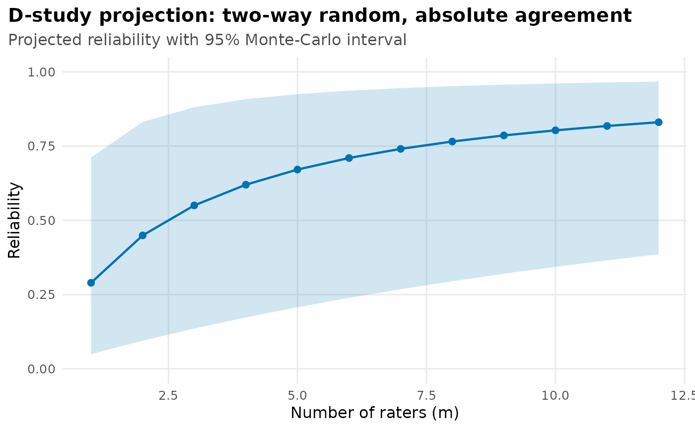
ggplot2::autoplot(d_study(fit_ag, m = 1:12)) # the D-study reliability curve
 fit <- icc(ratings, score, subject, rater, seed = 1)
d_study(fit, m = 1:8)
#> # D-study projection: two-way random, absolute agreement & consistency
#> Observed raters: 4 | CI: 95% montecarlo (10000 draws)
#> type m estimate 95% CI
#> agreement 1 0.290 [0.050, 0.706]
#> agreement 2 0.449 [0.096, 0.828]
#> agreement 3 0.550 [0.137, 0.878]
#> agreement 4 0.620 [0.175, 0.906]
#> agreement 5 0.671 [0.210, 0.923]
#> agreement 6 0.710 [0.241, 0.935]
#> agreement 7 0.741 [0.271, 0.944]
#> agreement 8 0.765 [0.298, 0.950]
#> consistency 1 0.715 [0.339, 0.924]
#> consistency 2 0.834 [0.507, 0.961]
#> consistency 3 0.883 [0.606, 0.973]
#> consistency 4 0.909 [0.672, 0.980]
#> consistency 5 0.926 [0.720, 0.984]
#> consistency 6 0.938 [0.755, 0.987]
#> consistency 7 0.946 [0.782, 0.988]
#> consistency 8 0.953 [0.804, 0.990]
fit <- icc(ratings, score, subject, rater, seed = 1)
d_study(fit, m = 1:8)
#> # D-study projection: two-way random, absolute agreement & consistency
#> Observed raters: 4 | CI: 95% montecarlo (10000 draws)
#> type m estimate 95% CI
#> agreement 1 0.290 [0.050, 0.706]
#> agreement 2 0.449 [0.096, 0.828]
#> agreement 3 0.550 [0.137, 0.878]
#> agreement 4 0.620 [0.175, 0.906]
#> agreement 5 0.671 [0.210, 0.923]
#> agreement 6 0.710 [0.241, 0.935]
#> agreement 7 0.741 [0.271, 0.944]
#> agreement 8 0.765 [0.298, 0.950]
#> consistency 1 0.715 [0.339, 0.924]
#> consistency 2 0.834 [0.507, 0.961]
#> consistency 3 0.883 [0.606, 0.973]
#> consistency 4 0.909 [0.672, 0.980]
#> consistency 5 0.926 [0.720, 0.984]
#> consistency 6 0.938 [0.755, 0.987]
#> consistency 7 0.946 [0.782, 0.988]
#> consistency 8 0.953 [0.804, 0.990]