library(tidyverse)
season <- c(1, 2, 3, 4, 5)
episodes <- c(7, 13, 13, 13, 16)
first_air <- c(2008, 2009, 2010, 2011, 2012)
last_air <- c(2008, 2009, 2010, 2011, 2013)
network <- "AMC"
breaking_bad <-
  tibble(season, episodes, first_air, last_air, network)

breaking_bad
## # A tibble: 5 × 5
##   season episodes first_air last_air network
##    <dbl>    <dbl>     <dbl>    <dbl> <chr>
## 1      1        7      2008     2008 AMC
## 2      2       13      2009     2009 AMC
## 3      3       13      2010     2010 AMC
## 4      4       13      2011     2011 AMC
## 5 5 16 2012 2013 AMCWeek 04: Wrangle
[04a] Tidy Data / Data Files
Topics
- Learn the principles of data storage and the tidy data format
- Read data from and write data to comma-separated values files
File Downloads
Readings
- R4DS (2E) Section 1.2.1: The penguins data frame
- R4DS (2E) Section 5.1: Data tidying - Introduction
- R4DS (2E) Section 5.2: Tidy data
- R4DS (2E) Section 7.2: Reading data from a file
- R4DS (2E) Section 7.5: Writing to a file
Slides
*Note that you can click the three-line (hamburger) icon on the bottom-left of the slides to access a navigation menu. You can click inside the slides region and press the left and right arrow keys on your keyboard to advance and reverse the slides and animations.
Practice
1) Tidy Data
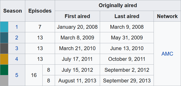
The following table summarizes the season information for the eight seasons of AMC’s Breaking Bad show.
Tidy up this data and save it to a tibble. Decide for yourself how to handle season 5 (should it be a single observation or two?). For the first and last aired dates, just store the year as a number.
Save the tibble you created to a CSV file in your Project folder named “breaking_bad.csv”.
Answer key
Version with one observation for the season five partsVersion with two separate observations for the season five parts
library(tidyverse)
season <- c(1, 2, 3, 4, 5.1, 5.2)
episodes <- c(7, 13, 13, 13, 8, 8)
first_air <- c(2008, 2009, 2010, 2011, 2012, 2013)
last_air <- c(2008, 2009, 2010, 2011, 2012, 2013)
network <- "AMC"
breaking_bad <-
  tibble(season, episodes, first_air, last_air, network)

breaking_bad
## # A tibble: 6 × 5
##   season episodes first_air last_air network
##    <dbl>    <dbl>     <dbl>    <dbl> <chr>
## 1    1          7      2008     2008 AMC
## 2    2         13      2009     2009 AMC
## 3    3         13      2010     2010 AMC
## 4    4         13      2011     2011 AMC
## 5    5.1        8      2012     2012 AMC
## 6    5.2        8      2013     2013 AMC
Part (b)
write_csv(breaking_bad, "breaking_bad.csv")
2) Data Files
Click the link to download the cereal.csv file and save it to your class Project folder.
Use {tidyverse} to import this file into R as a tibble named
cereal. Then print it.Use an R command to preview the data “at a glance.” How many variables and observations are in this tibble?
Answer key
Part (b)
cereal <- read_csv("cereal.csv")
cereal
## # A tibble: 77 × 8
##    name                      mfr       type  calories sodium carbo sugars rating
##    <chr>                     <chr>     <chr>    <dbl>  <dbl> <dbl>  <dbl> <chr>
##  1 100% Bran                 Nabisco   cold        70    130   5        6 68.40…
##  2 100% Natural Bran         Quaker O… cold       120     15   8        8 33.98…
##  3 All-Bran                  Kelloggs  cold        70    260   7        5 59.42…
##  4 All-Bran with Extra Fiber Kelloggs  cold        50    140   8        0 93.70…
##  5 Almond Delight            Ralston … cold       110    200  14        8 34.38…
##  6 Apple Cinnamon Cheerios   General … cold       110    180  10.5     10 29.50…
##  7 Apple Jacks               Kelloggs  cold       110    125  11       14 33.17…
##  8 Basic 4                   General … cold       130    210  18        8 37.03…
##  9 Bran Chex                 Ralston … cold        90    200  15        6 49.12…
## 10 Bran Flakes               Post      cold        90    210  13        5 53.31…
## # ℹ 67 more rows
Part (c)
glimpse(cereal)
## Rows: 77
## Columns: 8
## $ name     <chr> "100% Bran", "100% Natural Bran", "All-Bran", "All-Bran with …
## $ mfr      <chr> "Nabisco", "Quaker Oats", "Kelloggs", "Kelloggs", "Ralston Pu…
## $ type     <chr> "cold", "cold", "cold", "cold", "cold", "cold", "cold", "cold…
## $ calories <dbl> 70, 120, 70, 50, 110, 110, 110, 130, 90, 90, 120, 110, 120, 1…
## $ sodium   <dbl> 130, 15, 260, 140, 200, 180, 125, 210, 200, 210, 220, 290, 21…
## $ carbo    <dbl> 5.0, 8.0, 7.0, 8.0, 14.0, 10.5, 11.0, 18.0, 15.0, 13.0, 12.0,…
## $ sugars   <dbl> 6, 8, 5, 0, 8, 10, 14, 8, 6, 5, 12, 1, 9, 7, 13, 3, 2, 12, 13…
## $ rating   <chr> "68.402973", "33.983679", "59.425505", "93.704912", "34.38484…
77 observations (rows) and 8 variables (columns)
[04b] Rows / Columns
Topics
- Transform data by row using
arrange(),filter(), anddistinct() - Transform data by column using
mutate(),select(),rename(), andrelocate()
Readings
- R4DS (2E) Section 3.1: Data Transformation - Introduction
- R4DS (2E) Section 3.2: Data Transformation - Rows
- R4DS (2E) Section 3.3: Data Transformation - Columns
Slides
*Note that you can click the three-line (hamburger) icon on the bottom-left of the slides to access a navigation menu. You can click inside the slides region and press the left and right arrow keys on your keyboard to advance and reverse the slides and animations.
Practice
For both sets of questions, load and use the storms dataset from the dplyr package. Because changes are only saved when using assignment, be sure to use the <- in each line. Then print the final result.
1) Rows
Filter the
stormsdataset to show only the observations from the year 2005. Sort the result by pressure from lowest to highest (ascending) to see the most intense observations first.Use
distinct()to find the unique names of all storms in the dataset that have ever reached category 5.
Answer key
Part (a)
library(tidyverse)
data("storms", package = "dplyr")

storms_2005 <- filter(storms, year == 2005)
storms_2005 <- arrange(storms_2005, pressure)
storms_2005
## # A tibble: 873 × 13
##    name     year month   day  hour   lat  long status    category  wind pressure
##    <chr>   <dbl> <dbl> <int> <dbl> <dbl> <dbl> <fct>        <dbl> <int>    <int>
##  1 Wilma    2005    10    19    12  17.3 -82.8 hurricane        5   160      882
##  2 Wilma    2005    10    19     6  17   -82.2 hurricane        5   150      892
##  3 Wilma    2005    10    19    18  17.4 -83.4 hurricane        5   140      892
##  4 Wilma    2005    10    20     0  17.9 -84   hurricane        4   135      892
##  5 Rita     2005     9    22     3  24.7 -87.3 hurricane        5   155      895
##  6 Rita     2005     9    22     0  24.5 -86.9 hurricane        5   150      897
##  7 Rita     2005     9    22     6  24.8 -87.6 hurricane        5   155      897
##  8 Wilma    2005    10    20     6  18.1 -84.7 hurricane        4   130      901
##  9 Katrina  2005     8    28    18  26.3 -88.6 hurricane        5   150      902
## 10 Katrina  2005     8    29     0  27.2 -89.2 hurricane        5   140      905
## # ℹ 863 more rows
## # ℹ 2 more variables: tropicalstorm_force_diameter <int>,
## #   hurricane_force_diameter <int>
Part (b)
storms_cat5 <- filter(storms, category == 5)
storms_cat5 <- distinct(storms_cat5, name)
storms_cat5
## # A tibble: 25 × 1
##    name
##    <chr>
##  1 Anita
##  2 David
##  3 Allen
##  4 Gilbert
##  5 Hugo
##  6 Andrew
##  7 Mitch
##  8 Isabel
##  9 Ivan
## 10 Emily
## # ℹ 15 more rows
2) Columns
Create a subset of the
stormsdataset that contains only the name, year, and wind variables. Then, rename the wind column to max_wind_knots.Create a new column called wind_mph (wind * 1.15). Then, relocate this new column to appear immediately before the pressure column.
Answer key
Part (a)
storms_knots <- select(storms, name, year, wind)
storms_knots <- rename(storms_knots, max_wind_knots = wind)
storms_knots
## # A tibble: 20,778 × 3
##    name   year max_wind_knots
##    <chr> <dbl>          <int>
##  1 Amy    1975             25
##  2 Amy    1975             25
##  3 Amy    1975             25
##  4 Amy    1975             25
##  5 Amy    1975             25
##  6 Amy    1975             25
##  7 Amy    1975             25
##  8 Amy    1975             30
##  9 Amy    1975             35
## 10 Amy    1975             40
## # ℹ 20,768 more rows
Part (b)
storms_mph <- mutate(storms, wind_mph = wind * 1.15)
storms_mph <- relocate(storms_mph, wind_mph, .before = pressure)
storms_mph
## # A tibble: 20,778 × 14
##    name   year month   day  hour   lat  long status      category  wind wind_mph
##    <chr> <dbl> <dbl> <int> <dbl> <dbl> <dbl> <fct>          <dbl> <int>    <dbl>
##  1 Amy    1975     6    27     0  27.5 -79   tropical d…       NA    25     28.7
##  2 Amy    1975     6    27     6  28.5 -79   tropical d…       NA    25     28.7
##  3 Amy    1975     6    27    12  29.5 -79   tropical d…       NA    25     28.7
##  4 Amy    1975     6    27    18  30.5 -79   tropical d…       NA    25     28.7
##  5 Amy    1975     6    28     0  31.5 -78.8 tropical d…       NA    25     28.7
##  6 Amy    1975     6    28     6  32.4 -78.7 tropical d…       NA    25     28.7
##  7 Amy    1975     6    28    12  33.3 -78   tropical d…       NA    25     28.7
##  8 Amy    1975     6    28    18  34   -77   tropical d…       NA    30     34.5
##  9 Amy    1975     6    29     0  34.4 -75.8 tropical s…       NA    35     40.2
## 10 Amy    1975     6    29     6  34   -74.8 tropical s…       NA    40     46
## # ℹ 20,768 more rows
## # ℹ 3 more variables: pressure <int>, tropicalstorm_force_diameter <int>,
## #   hurricane_force_diameter <int>
[04c] Pipes / Pipelines
Topics
- Use the pipe (
|>) to efficiently pass an object to a function - Build a pipeline by connecting multiple pipes together
Readings
- R4DS (2E) Section 3.1.3: dplyr basics
- R4DS (2E) Section 3.4: The pipe
Slides
*Note that you can click the three-line (hamburger) icon on the bottom-left of the slides to access a navigation menu. You can click inside the slides region and press the left and right arrow keys on your keyboard to advance and reverse the slides and animations.
Practice
1) The Pipe
Rewrite the following “traditional” code using the native pipe operator.
- Nested Math: Rewrite this calculation to find the square root of 250, and then round the result to one decimal place.
# Traditional approach
round(sqrt(250), digits = 1)
## [1] 15.8- The Placeholder: Rewrite this repetition command. We want to repeat the word “Beetlejuice” exactly 3 times. Use the pipe to pass the number 3 into the times argument of the
rep()function.
# Traditional approach
rep("Beetlejuice", times = 3)
## [1] "Beetlejuice" "Beetlejuice" "Beetlejuice"
Answer key
Part (a)
250 |>
  sqrt() |>
  round(digits = 1)
## [1] 15.8
Part (b)
3 |>
  rep("Beetlejuice", times = _)
## [1] "Beetlejuice" "Beetlejuice" "Beetlejuice"
2) Pipelines
Write a single pipeline to answer the following question about breakfast cereals.
Question: Which cereals made by “General Mills” have high sugar content (greater than 10 grams)?
Requirements:
- Start by importing the data from the cereal.csv file
- Filter for the manufacturer (mfr) “General Mills” AND sugars greater than 10.
- Select only the name and sugars columns.
- Sort the results by sugars to place highest sugar at the top.
Answer key
# Note: Ensure cereal.csv is in your project folder
library(tidyverse)
read_csv("cereal.csv") |>
  filter(mfr == "General Mills", sugars > 10) |>
  select(name, sugars) |>
  arrange(desc(sugars))
## # A tibble: 5 × 2
##   name              sugars
##   <chr>              <dbl>
## 1 Total Raisin Bran     14
## 2 Cocoa Puffs           13
## 3 Count Chocula         13
## 4 Lucky Charms          12
## 5 Trix                  12