Week 12: Specialize

[12a] Strings

Topics

  • Understand how R handles strings and special characters
  • Combine, separate, and extract parts of text data
  • Use regular expressions to detect and replace patterns within strings

Readings

Slides

*Note that you can click the three-line (hamburger) icon on the bottom-left of the slides to access a navigation menu. You can click inside the slides region and press the left and right arrow keys on your keyboard to advance and reverse the slides and animations.

Practice

1) Combining and Extracting Text

Using the starwars dataset (included in {dplyr}), let’s generate descriptive text for each character.

  • First, use select() to keep just the name, species, and homeworld columns.
  • Use str_glue() inside a mutate() step to create a new column called description that dynamically inserts the character’s information into the string.
  • Create another column called home_abbr that uses str_sub() to extract only the first three letters of the character’s homeworld.

Answer key

library(tidyverse)

data("starwars", package = "dplyr")

starwars |> 
  select(name, species, homeworld) |> 
  mutate(
    description = str_glue("{name} is a {species} from {homeworld}."),
    home_abbr = str_sub(homeworld, start = 1, end = 3)
  )
## # A tibble: 87 × 5
##    name               species homeworld description                    home_abbr
##    <chr>              <chr>   <chr>     <glue>                         <chr>    
##  1 Luke Skywalker     Human   Tatooine  Luke Skywalker is a Human fro… Tat      
##  2 C-3PO              Droid   Tatooine  C-3PO is a Droid from Tatooin… Tat      
##  3 R2-D2              Droid   Naboo     R2-D2 is a Droid from Naboo.   Nab      
##  4 Darth Vader        Human   Tatooine  Darth Vader is a Human from T… Tat      
##  5 Leia Organa        Human   Alderaan  Leia Organa is a Human from A… Ald      
##  6 Owen Lars          Human   Tatooine  Owen Lars is a Human from Tat… Tat      
##  7 Beru Whitesun Lars Human   Tatooine  Beru Whitesun Lars is a Human… Tat      
##  8 R5-D4              Droid   Tatooine  R5-D4 is a Droid from Tatooin… Tat      
##  9 Biggs Darklighter  Human   Tatooine  Biggs Darklighter is a Human … Tat      
## 10 Obi-Wan Kenobi     Human   Stewjon   Obi-Wan Kenobi is a Human fro… Ste      
## # ℹ 77 more rows

2) Separating Product Codes

Data often comes with multiple pieces of information stored in a single column. Let’s practice splitting them apart using a simulated inventory dataset.

  • First, run the code provided below to create the inventory dataset.
  • Use separate_wider_delim() to split the item column into three separate columns: "furniture", "wood_type", and "price".
  • Set the delim argument to the hyphen character.
inventory <- tibble(
  item = c("Chair-Oak-199", "Table-Pine-299", "Desk-Birch-399")
)

Answer key

inventory |> 
  separate_wider_delim(
    cols = item,
    delim = "-",
    names = c("furniture", "wood_type", "price")
  )
## # A tibble: 3 × 3
##   furniture wood_type price
##   <chr>     <chr>     <chr>
## 1 Chair     Oak       199  
## 2 Table     Pine      299  
## 3 Desk      Birch     399

3) Regular Expressions

Let’s use regular expressions (regex) to find specific patterns in text and clean them up using building blocks like anchors and character classes.

  • Start with the starwars dataset and use filter() with str_detect() to find all characters whose name starts with either “A” or “S”. Hint: Use an anchor and a character class.
  • Use mutate() and str_remove_all() to create a new column called no_spaces that removes all whitespace from the names.
  • Select only the name and no_spaces columns to verify your work.

Answer key

starwars |> 
  filter(str_detect(name, "^[AS]")) |> 
  mutate(
    no_spaces = str_remove_all(name, "\\s")
  ) |> 
  select(name, no_spaces)
## # A tibble: 11 × 2
##    name             no_spaces      
##    <chr>            <chr>          
##  1 Anakin Skywalker AnakinSkywalker
##  2 Ackbar           Ackbar         
##  3 Arvel Crynyd     ArvelCrynyd    
##  4 Sebulba          Sebulba        
##  5 Shmi Skywalker   ShmiSkywalker  
##  6 Ayla Secura      AylaSecura     
##  7 Adi Gallia       AdiGallia      
##  8 Saesee Tiin      SaeseeTiin     
##  9 San Hill         SanHill        
## 10 Shaak Ti         ShaakTi        
## 11 Sly Moore        SlyMoore

[12b] Factors

Topics

  • Understand the difference between character strings and factors
  • Control the order of categorical data in plots and tables
  • Recode, collapse, and “lump” factor levels to simplify messy data

Readings

Slides

*Note that you can click the three-line (hamburger) icon on the bottom-left of the slides to access a navigation menu. You can click inside the slides region and press the left and right arrow keys on your keyboard to advance and reverse the slides and animations.

Practice

1) Ordering Factors by Value

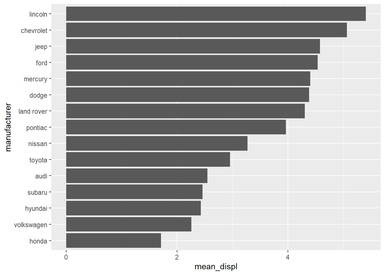
Using the mpg dataset (included in {ggplot2}), let’s create a bar chart that is ordered meaningfully instead of alphabetically.

  • First, calculate the average engine size (displ) for each manufacturer using summarize() and the .by argument. Name the new column mean_displ.
  • Use mutate() and fct_reorder() to reorder the manufacturer factor based on the calculated mean_displ.
  • Pipe the result into ggplot() and create a horizontal bar chart (geom_col()) with mean_displ on the x-axis and manufacturer on the y-axis.
  • Look at the plot to answer: which manufacturers make the largest and smallest engines on average?

Answer key

mpg |> 
  summarize(
    .by = manufacturer, 
    mean_displ = mean(displ)
  ) |> 
  mutate(
    manufacturer = fct_reorder(manufacturer, mean_displ)
  ) |> 
  ggplot(aes(x = mean_displ, y = manufacturer)) + 
  geom_col()

2) Lumping Rare Categories

When a categorical variable has too many levels, it can be helpful to group the smallest ones together.

  • Use the starwars dataset and drop any rows with a missing species value.
  • Use mutate() and fct_lump_n() to create a new column called species_lumped.
  • Keep only the top 3 most common species and lump all others into an “Other” category.
  • Pipe the result into count() to see the tallies for your new column.

Answer key

starwars |> 
  drop_na(species) |> 
  mutate(species_lumped = fct_lump_n(species, n = 3)) |> 
  count(species_lumped, sort = TRUE)
## # A tibble: 4 × 2
##   species_lumped     n
##   <fct>          <int>
## 1 Other             39
## 2 Human             35
## 3 Droid              6
## 4 Gungan             3

3) Collapsing Factor Levels

Sometimes we want to manually group specific categories together for a broader analysis

  • Using the diamonds dataset, create a new column called cut_simplified using fct_collapse().
  • Collapse “Ideal” and “Premium” into a single level called “Excellent”.
  • Collapse “Very Good”, “Good”, and “Fair” into a single level called “Standard”.
  • Run count() on your new cut_simplified column to see the results.

Answer key

diamonds |> 
  mutate(
    cut_simplified = fct_collapse(cut,
      "Excellent" = c("Ideal", "Premium"),
      "Standard"  = c("Very Good", "Good", "Fair")
    )
  ) |> 
  count(cut_simplified)
## # A tibble: 2 × 2
##   cut_simplified     n
##   <ord>          <int>
## 1 Standard       18598
## 2 Excellent      35342

[12c] Dates & Times

Topics

  • Parse strings and build dates from individual components
  • Extract, round, and modify date-time components
  • Understand periods, durations, and intervals for time spans

Readings

Slides

*Note that you can click the three-line (hamburger) icon on the bottom-left of the slides to access a navigation menu. You can click inside the slides region and press the left and right arrow keys on your keyboard to advance and reverse the slides and animations.

Practice

1) Parsing Dates from Strings

Let’s convert human-readable text into proper machine-readable dates.

  • Run the code below to load a small dataset of historical events.
  • Use mutate() and the appropriate {lubridate} parsing function to convert the date_str column into a proper Date object. Name the new column actual_date.
events <- tibble(
  event = c("Apollo 11 Landing", "First Flight", "Y2K Bug"),
  date_str = c("July 20, 1969", "December 17, 1903", "January 1, 2000")
)

Answer key

events |> 
  mutate(
    actual_date = mdy(date_str)
  )
## # A tibble: 3 × 3
##   event             date_str          actual_date
##   <chr>             <chr>             <date>     
## 1 Apollo 11 Landing July 20, 1969     1969-07-20 
## 2 First Flight      December 17, 1903 1903-12-17 
## 3 Y2K Bug           January 1, 2000   2000-01-01

2) Extracting Components

Using the economics dataset (including with {ggplot2}), let’s figure out which month historically has the highest average unemployment.

  • Use mutate() and month() to extract the month from the date column.
  • Set label = TRUE so you get the actual month label (e.g., “Jan”) instead of numbers.
  • Next, summarize() the average of the unemploy column grouped by your new month variable using .by.
  • Finally, arrange() the results in descending order to see the top months.

Answer key

economics |> 
  mutate(obs_month = month(date, label = TRUE)) |> 
  summarize(
    .by = obs_month,
    avg_unemploy = mean(unemploy)
  ) |> 
  arrange(desc(avg_unemploy))
## # A tibble: 12 × 2
##    obs_month avg_unemploy
##    <ord>            <dbl>
##  1 Jun              7838.
##  2 May              7800.
##  3 Apr              7799.
##  4 Feb              7789.
##  5 Mar              7787.
##  6 Jan              7780.
##  7 Nov              7770.
##  8 Dec              7760.
##  9 Jul              7736.
## 10 Oct              7735.
## 11 Aug              7735.
## 12 Sep              7727.

3) Calculating Time Spans

Let’s calculate exact lifespans using intervals and durations.

  • Run the code below to create a small dataset of early US Presidents.
  • Use mutate() and the interval() function to calculate the exact span of time between their born and died dates. Name this column life_span.
  • Create a final column called age_years by dividing the life_span interval by years(1) to see their age at death.
presidents <- tibble(
  name = c("George Washington", "Abraham Lincoln"),
  born = ymd(c("1732-02-22", "1809-02-12")),
  died = ymd(c("1799-12-14", "1865-04-15"))
)

Answer key

presidents |> 
  mutate(
    life_span = interval(start = born, end = died),
    age_years = life_span / years(1)
  )
## # A tibble: 2 × 5
##   name            born       died       life_span                      age_years
##   <chr>           <date>     <date>     <Interval>                         <dbl>
## 1 George Washing… 1732-02-22 1799-12-14 1732-02-22 UTC--1799-12-14 UTC      67.8
## 2 Abraham Lincoln 1809-02-12 1865-04-15 1809-02-12 UTC--1865-04-15 UTC      56.2