Modern Intraclass Correlation Coefficients • intraclass

intraclass computes interrater-reliability intraclass correlation coefficients (ICCs). An ICC is the share of the variation in scores that reflects real differences between the things rated, rather than rater noise. It works within the generalizability-theory framework, using modern variance-component estimation (linear mixed models) rather than the classical ANOVA / mean-squares approach.

It aims to fit variance components, each a share of the total variation traced to one source. It uses modern engines, an engine being the software that does the fitting. It aims to compute the correct ICC for a stated design. It gives a proper Monte-Carlo interval, built by drawing parameter values from the fitted model’s uncertainty. That interval is boundary-aware: an estimate can land exactly at zero, and the interval still behaves. It also aims to handle imbalanced, incomplete, and multilevel designs, and to help you decide which ICC to choose, and why. The docs and website are a place to learn ICC best practice, not only to look up functions.

The full interrater-reliability ICC family is implemented. That covers two-way designs, where each rater is tracked across the subjects they score, and one-way designs. Within two-way, it covers absolute agreement, where raters give the same score, against consistency, where raters agree apart from a constant offset per rater. It covers single-rater coefficients, the reliability of one rater’s score, and average-rater ones, the reliability of a mean of several raters. It covers random raters against fixed raters, where the observed raters are the whole population of interest. It covers imbalanced and incomplete (missing-cell) data. It also covers multilevel designs, where the subject level is reliability within a cluster, and the cluster level is reliability of cluster means. In such a design the raters may be crossed with or nested in clusters or subjects. Everything just listed comes with boundary-aware Monte-Carlo intervals. Fits run on glmmTMB (the default) or lme4. Bayesian fits run on brms, and SEM fits on lavaan. The engines article says which designs each one supports.

Installation

Install the released version from CRAN with:

install.packages("intraclass")

Or install the development version from GitHub with:

# install.packages("pak")
pak::pak("jmgirard/intraclass")

intraclass declares cli, generics, glmmTMB, lifecycle, rlang, and tibble as its non-base Imports:. What an installation retrieves is the full dependency closure of those declarations, which is considerably larger. One member of that closure is worth naming. glmmTMB lists lme4 in its own Imports:. So the lme4 package is already on your library path after a plain install, whatever its Suggests: placement here implies. Having the package is not the same as having the engine, though. engine = "lme4" also needs merDeriv, which every lme4 fit checks for on entry whatever interval method you ask for. merDeriv does not arrive. It sits in this package’s Suggests:, and so do brms, the Bayesian engine, and lavaan, the SEM engine. A plain install fetches none of the three. Asking for merDeriv does bring lavaan along, though, because merDeriv names it in its own Depends:. glmmTMB is the only engine a plain install leaves you ready to use.

Example

ratings is the classic Shrout & Fleiss (1979) example, shipped with the package. With the defaults a single two-way random fit reports every defined formulation: absolute agreement and consistency, single-rater and average. They are grouped by error definition, each with a reproducible Monte-Carlo interval:

library(intraclass)

fit <- icc(ratings, score, subject, rater, seed = 2024)
fit
#> ── Intraclass correlation: two-way random, absolute agreement & consistency ────
#> Subjects: 6 | Raters: 4 (random) | Observations: 24 of 24 cells (complete)
#> Engine: glmmTMB (REML) | CI: 95% montecarlo (10000 draws)
#> 
#>   index     estimate   95% CI
#>   Absolute agreement
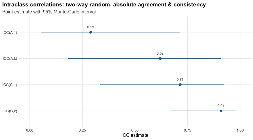
#>   ICC(A,1)     0.290   [0.053, 0.714]
#>   ICC(A,k)     0.620   [0.183, 0.909]
#>   Consistency
#>   ICC(C,1)     0.715   [0.334, 0.924]
#>   ICC(C,k)     0.909   [0.667, 0.980]
#> 
#> Variance components: subject 2.556, rater 5.244, residual 1.019
#> Shrout & Fleiss equivalent: ICC(A,1) = ICC(2,1), ICC(A,k) = ICC(2,k)

autoplot() draws the same fit as a forest plot (it needs ggplot2):

library(ggplot2)

autoplot(fit)

Forest plot of the four coefficients from the ratings fit: ICC(A,1), ICC(A,k), ICC(C,1) and ICC(C,k), each a labelled point with a horizontal Monte-Carlo interval, and the average-rater coefficients further to the right than their single-rater counterparts.

Which coefficient you want is a real modeling decision: agreement vs. consistency, single vs. average, fixed vs. random raters, complete vs. incomplete. Each of those is an argument to icc(). Not sure which to report? choose_icc() walks the Choosing an ICC decision tree. It hands back the coefficient or coefficients, the reasoning, and the exact call to run. No data or fitting is required:

choose_icc(model = "twoway", type = "consistency", unit = "average", raters = "random")
#> ── Recommended ICC ─────────────────────────────────────────────────────────────
#> Design: two-way random, consistency
#> 
#> Recommendation: ICC(C,k)
#> 
#> Why:
#>   - Crossed (two-way): the same raters judge every subject.
#>   - Consistency: only the rank order must match; a constant per-rater offset is forgiven.
#>   - Average: you will act on the mean of your raters.
#>   - Random raters: a sample you generalize beyond, to the rater universe they were drawn from.
#> 
#> Run this on your data:
#>   icc(data, score, subject, rater, type = "consistency", unit = "average")
#> 
#> Notes:
#>   - Complete vs. incomplete is automatic: icc() uses whatever ratings are present and projects ICC(*,k) to the effective number of ratings (k_eff). The design must stay connected, or icc() fails loudly.

For multilevel data, meaning subjects nested in clusters such as pupils in classrooms or patients in clinics, pass a cluster column. Then icc() reports subject-level and cluster-level reliability separately. The shipped school data are a simulated example, pupils nested in classrooms:

icc(school, score, subject = pupil, rater = rater, cluster = classroom, seed = 2024)
#> ℹ Treating raters with the same label in different clusters as the same raters
#>   (crossed with clusters, Design 1).
#> ℹ If each cluster has its own raters, give them cluster-unique labels or pass
#>   `design = "nested_in_clusters"`.
#> ── Intraclass correlation: multilevel two-way random, absolute agreement & consi
#> Subjects: 80 in 16 clusters | Raters: 4 (random) | Observations: 320 (complete)
#> Engine: glmmTMB (REML) | CI: 95% montecarlo (10000 draws)
#> 
#>   level      index     estimate   95% CI
#>   Absolute agreement
#>   subject    ICC(A,1)     0.431   [0.256, 0.565]
#>   subject    ICC(A,k)     0.751   [0.579, 0.838]
#>   cluster    ICC(A,1)     0.880   [0.000, 0.972]
#>   cluster    ICC(A,k)     0.967   [0.000, 0.993]
#>   Consistency
#>   subject    ICC(C,1)     0.493   [0.372, 0.615]
#>   subject    ICC(C,k)     0.796   [0.703, 0.865]
#>   cluster    ICC(C,1)     1.000   [0.000, 1.000]
#>   cluster    ICC(C,k)     1.000   [0.000, 1.000]
#> 
#> Variance components: cluster 0.998, subject 0.461, rater 0.136, cluster:rater 0.000, residual 0.473
#> 
#> This message is displayed once per session.

The cluster-level consistency rows sit on a boundary here: the classroom-by-rater variance is estimated at zero, so ICC(C,1) reaches 1 and its interval spans the whole range. The multilevel article (vignette("multilevel-designs")) explains what each level measures.

How many raters do you need?

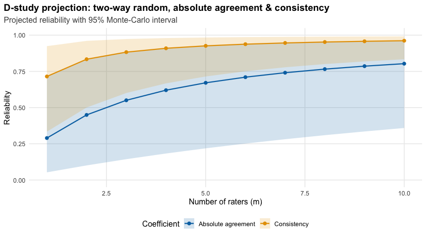
d_study() runs a D-study, which projects the fitted variance components to other rater or occasion counts, carrying the interval with them. So you can ask what reliability two raters would buy, or ten, without running the study again:

autoplot(d_study(fit, m = 1:10))

Projected reliability against the number of raters, from 1 to 10, as two rising curves with Monte-Carlo interval bands: consistency above, absolute agreement below, both climbing steeply from one to four raters and flattening after that.

Learn more

Getting started: the guided tour.
Choosing an ICC: the decision guide behind choose_icc().
Multilevel designs: incomplete and nested multilevel data.
Estimation engines: what each engine buys you.
Confidence-interval methods: the ci_method menu.
D-studies and replicates: projection, and replicates, each one of several ratings by the same rater of the same subject.
Comparison with other packages: how the numbers line up.
Glossary: the vocabulary in one place.

Citation

citation("intraclass")
#> To cite intraclass in publications use:
#> 
#>   Girard J (2026). _intraclass: Modern Intraclass Correlation
#>   Coefficients_. R package version 0.1.0.9000,
#>   <https://CRAN.R-project.org/package=intraclass>.
#> 
#> A BibTeX entry for LaTeX users is
#> 
#>   @Manual{intraclass,
#>     title = {{intraclass}: Modern Intraclass Correlation Coefficients},
#>     author = {Jeffrey Girard},
#>     year = {2026},
#>     note = {R package version 0.1.0.9000},
#>     url = {https://CRAN.R-project.org/package=intraclass},
#>   }
#> 
#> A companion software paper will be drafted at
#> https://github.com/jmgirard/intraclass-paper.

The companion software paper will be drafted in its own repository.

Contributing and support

Bug reports and questions are welcome on the issue tracker. The contributing guide says what to include, and why code contributions are not solicited.

Approach	Packages	What you get
Classical ANOVA / mean squares	`psych`, `irr`, `irrNA`, `irrICC`, `ICCDesign`	ANOVA / mean-squares based, mostly assuming balanced data
Model-based variance partition	`performance::icc`, `misty`	A variance-partition coefficient, but not the full interrater-reliability ICC family, the error-variance framing, or a selection framework
intraclass	(this package)	Mixed-model estimation, Monte-Carlo confidence intervals, and decision guidance

intraclass fills that gap, following ten Hove, Jorgensen & van der Ark.

intraclass