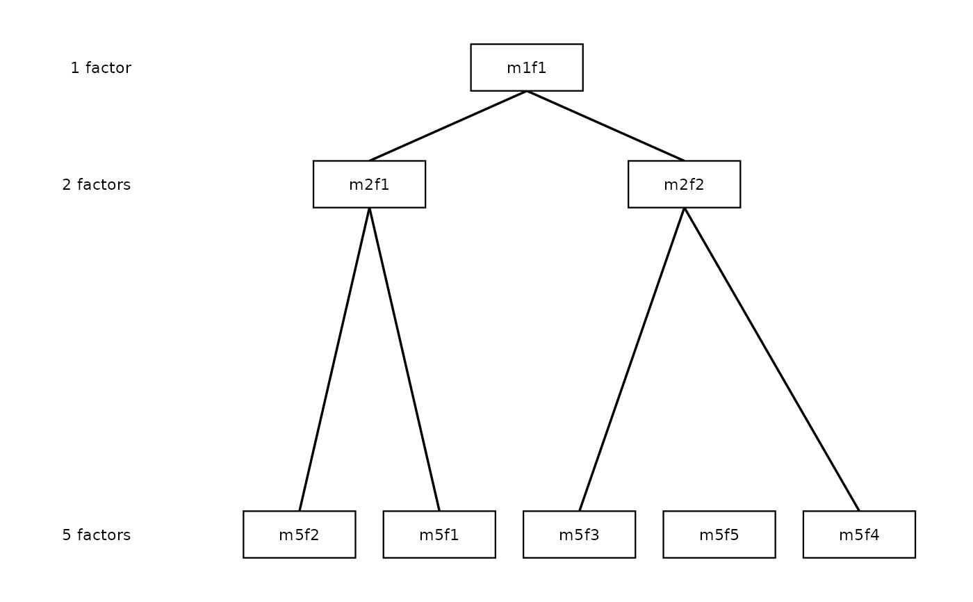
Plot a bass-ackwards diagram or per-level fit index chart

When what = "hierarchy" (default), renders the layered bass-ackwards hierarchy as a ggplot2 diagram. Factors appear as labelled boxes arranged in levels (level 1 at top, level k at bottom by default; set direction = "horizontal" for a left-to-right layout). Between-level edges below cut_show are hidden. Two aesthetics carry the edge information, each explained by its own legend: sign (positive/negative) is shown by sign_by (edge colour by default) and magnitude (|r|) by magnitude_by (line thickness by default). No aesthetic is ever mapped without a matching legend.

Usage

# S3 method for class 'ackwards'
autoplot(
  object,
  what = c("hierarchy", "fit"),
  sign_by = c("color", "linetype", "both", "none"),
  magnitude_by = c("linewidth", "none"),
  cut_show = NULL,
  color_pos = "#2166AC",
  color_neg = "#D6604D",
  color_edge = "black",
  colour_pos = NULL,
  colour_neg = NULL,
  colour_edge = NULL,
  node_width = 0.8,
  node_height = 0.4,
  min_sep = 1,
  order = NULL,
  show_items = FALSE,
  n_items = 5,
  item_cut = 0.3,
  show_skip = NULL,
  curvature = 0.2,
  color_pruned = "grey80",
  colour_pruned = NULL,
  show_r = FALSE,
  r_digits = 2L,
  r_label_size = 2.5,
  mono = FALSE,
  edge_linewidth = NULL,
  cut_strong = NULL,
  direction = c("vertical", "horizontal"),
  show_level_labels = TRUE,
  level_label_size = 3,
  node_labels = NULL,
  primary_only = FALSE,
  drop_pruned = FALSE,
  compress_levels = FALSE,
  show_secondary = FALSE,
  show_arrows = TRUE,
  legend = TRUE,
  ...
)

# S3 method for class 'ackwards'
plot(x, ...)

Arguments

object: An ackwards object.
what: One of "hierarchy" (default) or "fit". Controls which visualisation is produced. All other parameters are ignored when what = "fit".
sign_by: How edge sign (positive vs negative correlation) is encoded. One of "color" (default; positive = color_pos, negative = color_neg), "linetype" (positive = solid, negative = dashed), "both" (colour and linetype, with negative drawn as a distinct double-dash so it reads clearly in greyscale), or "none" (sign not encoded; all edges color_edge and solid). Whichever channel is used gets a "Direction" legend. Colour is the default because it reads sign pre-attentively and leaves linetype free; switch to "linetype" or "both" for greyscale or colour-blind-safe figures.
magnitude_by: How edge magnitude (|r|) is encoded. One of "linewidth" (default; thicker = stronger, with a |r| legend) or "none" (constant width). A numeric edge_linewidth also forces constant width at that value.
cut_show: Edges with |r| < cut_show are not drawn. Defaults to the value used when the object was created (x$meta$cut_show, typically 0.3).
color_pos, colour_pos: Colour for positive edges when sign_by uses colour. Default "#2166AC" (blue). colour_pos is an accepted British alias.
color_neg, colour_neg: Colour for negative edges when sign_by uses colour. Default "#D6604D" (red). colour_neg is an accepted British alias.
color_edge, colour_edge: Single colour for all edges when sign_by does not use colour ("linetype" or "none"). Default "black". colour_edge is an accepted British alias.
node_width: Width of factor boxes in layout units. Either a single value applied to every box (default 0.8), or a named numeric vector keyed by factor ID (e.g. c(m5f1 = 1.6)) giving a per-box width; boxes not named fall back to the 0.8 default. Use a per-box width to fit a long manual node_labels string. Names matching no factor ID warn.
node_height: Height of factor boxes in layout units. Either a single value applied to every box (default 0.4), or a named numeric vector keyed by factor ID for a per-box height (unnamed boxes fall back to 0.4); useful for multi-line manual labels. Names matching no factor ID warn.
min_sep: Minimum horizontal separation between nodes; passed to ba_layout(). Default 1.0.
order: Optional manual left-to-right ordering of the deepest (k_max) level, passed to ba_layout(); a character vector of that level's factor IDs (or a named list keyed by the level number) fixes the leaf order and every upper factor re-centres above its primary children. Use it to untangle a figure by hand. NULL (default) uses the automatic ordering.
show_items: When TRUE, lists the salient observed items beneath each deepest-level (k_max) factor box, so a publication figure shows what each most-granular factor is made of. Items are the top n_items by |loading| at or above item_cut, using the same extraction as top_items() (variable labels are shown when the fit carried them, else the item IDs). Listed below the boxes in a vertical layout, to their right in a horizontal one. Default FALSE.
n_items: Maximum number of items listed per deepest-level factor when show_items = TRUE. NULL lists every item meeting item_cut. Default 5.
item_cut: Absolute-loading threshold for show_items: only items with |loading| >= item_cut are listed. Default 0.3.
show_skip: Whether to draw skip-level (non-adjacent) edges. NULL (default) auto-detects: TRUE when the object was run with pairs = "all", FALSE otherwise. Ignored when drop_pruned = TRUE.
curvature: Curvature of skip-level edge arcs. Passed to ggplot2::geom_curve(). Positive values curve right; default 0.2. Ignored when drop_pruned = TRUE.
color_pruned, colour_pruned: Fill colour for nodes flagged as pruned/redundant. Default "grey80". Only applied when the object carries pruning annotations (x$prune is non-NULL) and drop_pruned = FALSE (pruned nodes are omitted entirely when drop_pruned = TRUE). colour_pruned is an accepted British alias.
show_r: Whether to label each drawn edge with its correlation coefficient. Default FALSE. When TRUE, labels are formatted in APA style (leading zero stripped, e.g. .23, -.30) and placed beside each edge using a white-background label that clears the arrowhead.
r_digits: Number of decimal places for edge labels when show_r = TRUE. Default 2L.
r_label_size: Font size for edge correlation labels when show_r = TRUE. Passed to ggplot2::geom_label() as size. Default 2.5.
mono: Monochrome convenience wrapper. When TRUE, equivalent to sign_by = "linetype" with black edges (it overrides sign_by and the colour arguments). magnitude_by still applies. Default FALSE.
edge_linewidth: NULL (default) uses magnitude_by to decide edge width. A numeric value forces every edge to that constant width (implying magnitude_by = "none") and drops the |r| legend. Forbes figures use uniform thin lines (~= 0.5–0.6).
cut_strong: Deprecated in M35 and ignored (with a warning). Edge magnitude is now shown by magnitude_by (linewidth) and sign by sign_by; the old strong/weak linetype split double-encoded magnitude. Retained only so existing calls do not error.
direction: Layout orientation. "vertical" (default) stacks levels top-to-bottom (level 1 at top); "horizontal" lays them out left-to-right (level 1 at left), which suits wide slides or posters. Level-axis labels move to the bottom margin under "horizontal".
show_level_labels: Whether to draw level axis labels ("1 factor", "2 factors", ...) to the left of the diagram. Default TRUE. When the object carries pruning annotations (x$prune non-NULL) and drop_pruned = FALSE, a level whose factors are all pruned has its axis label rendered in italic to denote its status (matching the grey node fill); partially-pruned levels keep a plain label.
level_label_size: Font size for level axis labels. Default 3.
node_labels: A named character vector mapping factor IDs (e.g. "m5f1") to custom display strings (e.g. "General"). Unspecified factors keep any label attached with set_factor_labels(), falling back to the default m{k}f{j} ID. Entries here override a stored factor label for that node, so this argument is a per-call last word over the persistent labels. A warning is issued for names that match no factor ID in the object. Default NULL.
primary_only: When TRUE, only primary-parent edges (is_primary == TRUE) are drawn. Because skip-level edges are never primary, this also suppresses skip arcs. Ignored when drop_pruned = TRUE. Default FALSE.
drop_pruned: When TRUE, activates the Forbes (2023) pruned-view rendering path: pruned nodes are removed from the diagram entirely and each retained node is connected to its single strongest kept ancestor by a straight arrow (even across level gaps). Requires the object to carry pruning annotations (piped through prune()); errors if not. Overrides show_skip, curvature, and primary_only. Default FALSE.
compress_levels: When TRUE under drop_pruned = TRUE, closes vertical gaps left by pruned levels so retained levels are evenly spaced; level axis labels (d) still show the original level numbers. Ignored when drop_pruned = FALSE. Default FALSE.
show_secondary: When TRUE under drop_pruned = TRUE, also draws the between-level correlation edges the single-strongest-ancestor primary view hides: every kept cross-level factor pair with |r| >= cut_show that is not already a primary edge. This includes cross-branch second parents and same-lineage skip arcs (a direct skip-level r is a distinct, non-transitive fact, not implied by the primary path). Secondary edges render in a channel deliberately distinct from the primary edges – dimmed (reduced opacity) and thinner, with plain line ends – while still inheriting the sign encoding (sign_by), so the sign colour/linetype is never conflated with the secondary channel. By construction each node's secondaries are weaker than its primary edge, so a secondary edge never appears while that node's primary is below cut_show. Ignored when drop_pruned = FALSE. Default FALSE.
show_arrows: When FALSE, edges are drawn with plain line ends instead of closed arrowheads (arrow = NULL). Applies to both straight and curved edge layers. Default TRUE. Forbes (2023) figures use plain line ends.
legend: When FALSE, suppresses all plot legends (legend.position = "none"). Useful when color_pos == color_neg (e.g. both "black") to remove an otherwise redundant Direction key. Default TRUE.
...: Ignored.
x: An ackwards object.

Value

A ggplot object.

Details

When what = "fit", renders a two-panel line plot of per-level fit indices (CFI/TLI in the top panel; RMSEA/SRMR in the bottom panel) with horizontal reference lines at conventional Hu & Bentler (1999) thresholds. The anchor level (k = 1, saturated and always fits perfectly) is excluded. Requires an EFA or ESEM engine; returns an informative empty plot for PCA (which has no model-fit indices).

Requires the ggplot2 package.

Saving plots

autoplot() returns a standard ggplot object, so save it with ggplot2::ggsave():


  p <- autoplot(x)
  ggplot2::ggsave("hierarchy.png", p, width = 8, height = 6, dpi = 300)

ggsave() is not re-exported by ackwards (that would move ggplot2 from Suggests into Imports); call it from ggplot2 directly. For a wide slide or poster, pair it with direction = "horizontal".

Examples

# \donttest{
if (requireNamespace("ggplot2", quietly = TRUE)) {
  # sim16 has a known 1 -> 2 -> 4 hierarchy (continuous; pearson basis)
  x <- ackwards(sim16, k_max = 5)
  autoplot(x)
  autoplot(x, color_pos = "steelblue")

  # Encode sign by linetype instead of colour, or by both
  autoplot(x, sign_by = "linetype")
  autoplot(x, sign_by = "both")

  # Left-to-right layout (wide slides / posters)
  autoplot(x, direction = "horizontal")

  # List the top items under each deepest-level factor
  autoplot(x, show_items = TRUE, n_items = 4)

  # Per-level fit index chart (EFA or ESEM only)
  x_efa <- ackwards(sim16, k_max = 5, engine = "efa")
  autoplot(x_efa, what = "fit")

  # Monochrome with correlation labels (for greyscale figures)
  autoplot(x, mono = TRUE, show_r = TRUE)

  # Custom node labels for the 5-factor level
  autoplot(x, node_labels = c(m5f1 = "Factor A", m5f2 = "Factor B"))

  # Widen two boxes to fit long manual labels (per-box sizing)
  autoplot(x,
    node_labels = c(m5f1 = "Conscientiousness"),
    node_width = c(m5f1 = 1.8)
  )

  # Primary links only -- clean hierarchy tree
  autoplot(x, primary_only = TRUE)

  # Manually order the deepest level to untangle the figure by hand
  ids5 <- paste0("m5f", c(2, 1, 3, 5, 4))
  autoplot(x, order = ids5)

  # Forbes pruned view: omit redundant nodes, straight spanning arrows
  xp <- ackwards(sim16, k_max = 5) |> prune("redundant")
  autoplot(xp, drop_pruned = TRUE)
  autoplot(xp, drop_pruned = TRUE, show_r = TRUE)
  autoplot(xp, drop_pruned = TRUE, compress_levels = TRUE)

  # Add the secondary between-level correlations the primary view hides
  # (dimmed + thinner, drawn beneath the primary edges)
  autoplot(xp, drop_pruned = TRUE, show_secondary = TRUE)

  # Plain line ends without arrowheads
  autoplot(x, show_arrows = FALSE)

  # Uniform edge width (no |r| scaling)
  autoplot(x, edge_linewidth = 0.5)

  # Suppress legend
  autoplot(x, legend = FALSE)

  # Forbes (2023) publication style: black lines, uniform width, no arrowheads
  autoplot(xp,
    drop_pruned = TRUE,
    color_pos = "black", color_neg = "black",
    edge_linewidth = 0.6, show_arrows = FALSE, legend = FALSE
  )
}
#> Warning: `min_sep` (1) is less than the widest box (1.8); adjacent boxes may overlap.
#> ℹ Redundancy pruning (direct criterion, |r| ≥ 0.9) flagged 7 nodes.
#> ℹ Nodes are retained in the object; inspect with `x$prune$nodes` and
#>   `x$prune$chains`.

# }