Introduction to Bass-Ackwards Analysis

The problem: which solution is right?

A factor is an unobserved dimension that explains why a set of items correlate. Anyone who runs a factor analysis faces the same question: how many factors should you extract? Parallel analysis, a criterion that keeps a factor only when it explains more variance than random data would, might say 5. The scree plot might suggest 3. A reviewer might insist on 1. Each solution seems to describe the data differently, and it is tempting to treat them as competing answers to the same question.

Goldberg (2006) reframed this problem. The different solutions are not competing. They are complementary. A 1-factor solution captures the broadest shared variance in the data, the dimension along which all variables correlate. A 5-factor solution captures narrower, more specific dimensions. These two levels of resolution describe the same underlying structure from different vantage points, just as a satellite image and a street map describe the same city.

The bass-ackwards method makes this relationship explicit. It fits factor models at every level from 1 up to k. It then computes the correlations between factor scores across adjacent levels. A factor score is each person’s estimated position on a factor. Those correlations show you three things:

Which narrow factor inherits from which broad factor. This is the lineage of each dimension as you move from coarse to fine resolution.
Where a factor splits. A single broad factor that correlates strongly with two narrower factors is fragmenting into sub-dimensions.
Where a factor is stable. A factor that correlates about 1.0 with its counterpart at the adjacent level is the same construct appearing at two resolutions.

The result is a hierarchy map, a visual and numerical account of how the factor structure of your data builds from broad to narrow.

Note: This is a descriptive, data-driven hierarchy, not a confirmatory hierarchical model like Schmid-Leiman or higher-order SEM. The between-level correlations are score correlations (or their algebraic equivalents), not model parameters.

Data

We use bfi25, the built-in 25-item Big Five example dataset. The items measure five personality traits: Agreeableness (A1 to A5), Conscientiousness (C1 to C5), Extraversion (E1 to E5), Neuroticism (N1 to N5), and Openness (O1 to O5). Each item uses a 6-point Likert scale. See ?bfi25 for full provenance. The data derive from the SAPA project using public-domain IPIP items.

library(ackwards)

bfi <- na.omit(bfi25)
dim(bfi)
#> [1] 875  25

We drop cases with any missing item. In a real analysis you might use pairwise deletion or multiple imputation. For this illustration, na.omit() is enough.

Step 1: How many factors? `suggest_k()`

Before fitting the hierarchy, get a sense of the plausible range of k. suggest_k() runs five complementary selection criteria and reports a consensus range:

sk <- suggest_k(bfi, seed = 42)
#> ℹ Running parallel analysis (20 iterations, PC + FA)...
#> ✔ Running parallel analysis (20 iterations, PC + FA)... [93ms]
#> 
#> ℹ Running MAP and VSS...
#> ✔ Running MAP and VSS... [30ms]
#> 
#> ℹ Running Comparison Data (CD)...
#> ✔ Running Comparison Data (CD)... [3.9s]
#> 
print(sk)
#> 
#> ── Factor / Component Count Suggestion (ackwards) ──────────────────────────────
#> Variables: 25
#> n: 875
#> Basis: pearson
#> Tested k: 1-8
#> 
#> ── Criteria (k = 1-8) ──
#> 
#>   k  PA-PC  PA-FA      MAP    VSS-1    VSS-2  CD
#>   1     ✔︎      ✔︎   0.0254   0.5178   0.0000   ✔︎ 
#>   2     ✔︎      ✔︎   0.0194   0.5839   0.6719   ✔︎ 
#>   3     ✔︎      ✔︎   0.0175   0.5913   0.7354   ✔︎ 
#>   4     ✔︎      ✔︎   0.0164   0.6215*  0.7837   ✔︎ 
#>   5     ✔︎      ✔︎   0.0160*  0.5738   0.7950*  ✔︎ 
#>   6     -      ✔︎   0.0172   0.5594   0.7629   ✔︎*
#>   7     -      -   0.0205   0.5613   0.7616   - 
#>   8     -      -   0.0236   0.5600   0.7215   -
#>   ✔︎ retained   * optimal k   - not retained
#> 
#> ── Recommendations ──
#> 
#> • PA-PC: k <= 5
#> • PA-FA: k <= 6
#> • MAP: k = 5
#> • VSS-1: k = 4
#> • VSS-2: k = 5
#> • CD: k = 6
#> Consensus range: k = 4-6
#> ────────────────────────────────────────────────────────────────────────────────
#> Note: k_max in ackwards() is a maximum depth. Setting k_max one or two levels
#> above the consensus to observe factor fragmentation is intentional.
#> Caution: PA-PC tends to overextract; structures may not replicate (Forbes,
#> 2023). PA-FA and CD are more conservative. Use the range.

autoplot(sk)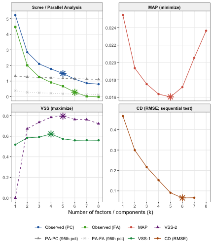

plot of chunk suggest_k_plot

suggest_k() does not return a single “correct” k. It reports what several criteria each recommend, so you can read a plausible range rather than a point estimate. It also warns that these items look ordinal, which means they are recorded on an ordered scale with a small number of categories. suggest_k() screens on the Pearson basis by design. Its warning therefore points you at cor = "polychoric" for the final fit, which we use in Step 2, and not at suggest_k() itself. That range informs k_max in ackwards(). k_max is an upper bound on the hierarchy depth, not a claim about the true number of factors. Setting k_max one or two levels above the consensus to watch factors fragment is intentional and informative. Before you interpret those deeper levels, gate them on replicability with comparability(). The recommended-workflow vignette, vignette("ackwards-girard"), is built around exactly this. For a full explanation of each criterion, its bias direction, and how to match it to your engine, see vignette("ackwards-suggest-k").

Step 2: Fit the hierarchy `ackwards()`

Now fit the bass-ackwards hierarchy. The most important arguments are:

Argument	What it controls	Default
`k_max`	Maximum depth of the hierarchy	(required)
`engine`	Extraction engine: `"pca"`, `"efa"`, or `"esem"`	`"pca"`
`cor`	Correlation type: `"pearson"`, `"spearman"`, `"polychoric"`	`"pearson"`

The default engine is PCA (principal component analysis), which summarizes the items with weighted sums called components. EFA (exploratory factor analysis) instead models the items as a small number of shared factors plus item-specific noise. ESEM (exploratory structural equation modeling) fits that same factor model in lavaan and adds standard errors. All three report loadings. A loading is the correlation between an item and a factor. The engines are compared in vignette("ackwards-engines").

Because BFI items are ordinal, we use cor = "polychoric". A polychoric correlation estimates the correlation between two ordinal items as if each were a continuous variable cut into categories. Computing these correlations before factor extraction gives a more accurate representation of the latent structure.

x <- ackwards(bfi, k_max = 5, cor = "polychoric")

ackwards() does not repeat the ordinal-detection warning that suggest_k() raised. Setting cor = "polychoric" is exactly how you heed it. It tells ackwards() that you have accounted for the ordinal measurement scale.

Why varimax? A rotation re-orients the factors within a level without changing how well they fit. Within each level, ackwards() rotates the factors orthogonally using varimax, which pushes each item toward one factor and keeps the factors uncorrelated. This is not merely a cosmetic default. The reason is not numerical: the W′RW between-level correlation identity is exact for any fixed linear scoring, oblique included. The reason is interpretive. Varimax leaves the factors within a level uncorrelated (Φ = I), so a between-level score correlation reflects only the cross-level relationship. Under an oblique rotation the within-level factors are themselves correlated (Φ ≠ I), and that within-level correlation leaks into the between-level edges. It confounds the within-versus-between question the method exists to answer. That confound is why the package does not offer oblique rotations. Varimax is the orthogonal rotation Goldberg (2006) used. It is also the same rotation as the “CF-VARIMAX” reported by Mplus-based papers such as Kim & Eaton (2015), because CF(κ = 1/p) is varimax. The two labels are not competing choices.

Step 3: Summarize the result

High-level summary

print() gives a quick overview:

print(x)
#> 
#> ── Bass-Ackwards Analysis (ackwards) ───────────────────────────────────────────
#> Engine: pca
#> Rotation: varimax
#> Basis: polychoric
#> n: 875
#> k (max): 5
#> 
#> ── Levels ──
#> 
#> ✔ k = 1: 1 factor, 23.2% variance
#> ✔ k = 2: 2 factors, 35.5% variance
#> ✔ k = 3: 3 factors, 44.6% variance
#> ✔ k = 4: 4 factors, 52.2% variance
#> ✔ k = 5: 5 factors, 58.4% variance
#> 
#> ── Edges ──
#> 
#> 14 of 40 edges have |r| ≥ 0.3
#> ────────────────────────────────────────────────────────────────────────────────
#> Note: This is a series of linked solutions, not a fitted hierarchical model.
#> Cross-level edges are descriptive score correlations. Per-level fit indices
#> (EFA/ESEM) describe how well a k-factor model fits the items at that level --
#> they do not validate the edges or the hierarchy itself.

The “Levels” section confirms that all five models converged. It also reports the cumulative variance explained at each level. Notice that the jump from k = 1 to k = 2 is large (from 23.2% to 35.5%), while later jumps are smaller. That pattern is characteristic of data with a strong general factor and several specific dimensions.

The “Edges” section reports how many of the 40 possible between-level connections exceed the display threshold of |r| ≥ 0.3. The 40 comes from summing across all adjacent pairs: 1×2 + 2×3 + 3×4 + 4×5 = 2 + 6 + 12 + 20 = 40.

summary() gives a more detailed view. It reports per-factor variance and fit indices at each level, plus a lineage list showing which factors at each level descend from which parents:

summary(x)
#> 
#> ── Summary: Bass-Ackwards Analysis (ackwards) ──────────────────────────────────
#> Engine: pca
#> Rotation: varimax
#> Basis: polychoric
#> n: 875
#> k (max): 5
#> 
#> ── Levels ──
#> 
#> k = 1: 1 factor (23.2% cumulative variance)
#> m1f1 23.2% eigenvalue 5.80
#> 
#> k = 2: 2 factors (35.5% cumulative variance)
#> m2f1 20.9% eigenvalue 5.80
#> m2f2 14.5% eigenvalue 3.07
#> 
#> k = 3: 3 factors (44.6% cumulative variance)
#> m3f1 18.0% eigenvalue 5.80
#> m3f2 13.9% eigenvalue 3.07
#> m3f3 12.7% eigenvalue 2.28
#> 
#> k = 4: 4 factors (52.2% cumulative variance)
#> m4f1 17.5% eigenvalue 5.80
#> m4f2 13.6% eigenvalue 3.07
#> m4f3 11.8% eigenvalue 2.28
#> m4f4 9.2% eigenvalue 1.90
#> 
#> k = 5: 5 factors (58.4% cumulative variance)
#> m5f1 13.8% eigenvalue 5.80
#> m5f2 13.6% eigenvalue 3.07
#> m5f3 11.9% eigenvalue 2.28
#> m5f4 10.1% eigenvalue 1.90
#> m5f5 9.1% eigenvalue 1.56
#> 
#> ── Lineage (primary parents) ──
#> 
#> m1f1 → m2f1, m2f2
#> m2f1 → m3f1, m3f3
#> m2f2 → m3f2
#> m3f1 → m4f1
#> m3f2 → m4f2
#> m3f3 → m4f3, m4f4
#> m4f1 → m5f1, m5f4
#> m4f2 → m5f2
#> m4f3 → m5f3
#> m4f4 → m5f5
#> ────────────────────────────────────────────────────────────────────────────────
#> Note: This is a series of linked solutions, not a fitted hierarchical model.
#> Cross-level edges are descriptive score correlations. Per-level fit indices
#> (EFA/ESEM) describe how well a k-factor model fits the items at that level --
#> they do not validate the edges or the hierarchy itself.

glance() returns the same top-level information as a one-row data frame, which is convenient for comparisons across models:

glance(x)
#>   engine rotation        cor k_max n_obs deepest_converged n_edges CFI TLI
#> 1    pca  varimax polychoric     5   875                 5      40  NA  NA
#>   RMSEA SRMR BIC
#> 1    NA   NA  NA

Step 4: Visualize the hierarchy `autoplot()`

The hierarchy diagram is the centerpiece of the method. Each row represents one level (k = 1 at the top, k = 5 at the bottom). Arrows connect each factor to its primary parent, the factor at the level above with which it has the strongest correlation (|r|). Arrow thickness is proportional to |r|, and color shows direction (blue = positive, red = negative by default). Both aesthetics come with a legend. In this clean solution every drawn edge is positive, so only blue appears here. For a left-to-right layout (handy for wide slides), pass direction = "horizontal".

autoplot(x)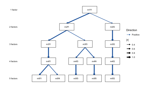

plot of chunk autoplot

Reading this diagram from broad (top) to narrow (bottom) tells the story of the Big Five:

k = 1: One broad factor. Given the polychoric basis, this captures shared variance across all 25 items.
k = 2: The broad factor splits into two. Neuroticism separates from a mixed cluster of Extraversion, Agreeableness, Conscientiousness, and Openness items (Extraversion items load most strongly within that cluster).
k = 3: The non-Neuroticism cluster splits again, separating Extraversion/Agreeableness from Conscientiousness/Openness. Neuroticism stays intact and sheds its residual cross-loadings.
k = 4: Conscientiousness and Openness differentiate into their own factors.
k = 5: Extraversion and Agreeableness finally differentiate, completing the canonical Big Five.

The factors are labeled m{k}f{j} (level k, factor j). These stable IDs are used throughout the object. So m5f1 at k = 5 refers to the same factor in the loadings, the edge table, the factor scores, and the diagram.

Adjusting the diagram

autoplot() accepts arguments to control edge thresholds, colours, line styles, arrowheads, node labels, and more. See vignette("ackwards-visualization") for a guided tour of all options with rendered examples, or ?autoplot.ackwards for the full argument list.

Step 5: Dig into the factors `tidy()`

tidy() extracts any part of the result as a tidy data frame. The what argument controls what is returned.

Reading each factor with `top_items()`

To understand what each factor represents, top_items() lists the salient items for every factor, grouped by level. An item is salient when its loading, the correlation between the item and the factor, is at least cut in absolute value. This is more readable than a full item-by-factor matrix, especially for deep hierarchies.

top_items(x, level = 5, cut = 0.5)
#> 
#> ── Salient items by factor (ackwards) ──────────────────────────────────────────
#> Engine: pca
#> Cut: |loading| >= 0.5
#> Top-n: all
#> 
#> ── Level 5 (5 factors) ──
#> 
#> m5f1
#> E2 [-0.752]
#> E4 [0.747]
#> E1 [-0.701]
#> E3 [0.677]
#> E5 [0.597]
#> 
#> m5f2
#> N3 [-0.825]
#> N1 [-0.810]
#> N2 [-0.805]
#> N5 [-0.688]
#> N4 [-0.646]
#> 
#> m5f3
#> C2 [0.735]
#> C4 [-0.716]
#> C1 [0.690]
#> C3 [0.679]
#> C5 [-0.652]
#> 
#> m5f4
#> A1 [-0.704]
#> A3 [0.703]
#> A2 [0.692]
#> A5 [0.580]
#> A4 [0.522]
#> 
#> m5f5
#> O5 [-0.705]
#> O3 [0.655]
#> O1 [0.604]
#> O2 [-0.595]
#> O4 [0.551]
#> ────────────────────────────────────────────────────────────────────────────────
#> Loadings reflect primary-parent sign alignment. Use tidy(x, what = "loadings")
#> for the full matrix.

Reading a hierarchy of factors and giving them names is its own topic. It covers the sign convention, naming across levels, and applying labels to the diagram. See vignette("ackwards-interpret") for the full workflow.

Factor loadings (tidy)

For programmatic access, tidy(what = "loadings") returns the full loading matrix in long format, with one row per item × factor × level:

loadings_df <- tidy(x, what = "loadings")
head(loadings_df)
#>   level factor item    loading se ci_lower ci_upper
#> 1     1   m1f1   A1 -0.3440908 NA       NA       NA
#> 2     1   m1f1   A2  0.5977210 NA       NA       NA
#> 3     1   m1f1   A3  0.6511387 NA       NA       NA
#> 4     1   m1f1   A4  0.4837850 NA       NA       NA
#> 5     1   m1f1   A5  0.6848262 NA       NA       NA
#> 6     1   m1f1   C1  0.4502778 NA       NA       NA

The se, ci_lower, and ci_upper columns are NA here. PCA (and EFA) return point loadings with no standard errors, so there is nothing to report. These columns are populated only by engine = "esem", which fits each level in lavaan and can attach model-based standard errors and confidence intervals to the loadings. See vignette("ackwards-engines").

Between-level edges

Each edge is the between-level factor-score correlation computed with Waller’s (2007) closed-form W′RW algebra. That is an exact result that requires no score materialization, just the weight matrices and the input correlation matrix.

# Each factor's primary-parent edge, strongest first
tidy(x, what = "edges", primary_only = TRUE, sort = "strength")
#>    from   to level_from level_to         r      beta is_primary above_cut
#> 1  m4f2 m5f2          4        5 0.9984791 0.9984791       TRUE      TRUE
#> 2  m3f1 m4f1          3        4 0.9938371 0.9938371       TRUE      TRUE
#> 3  m4f4 m5f5          4        5 0.9894063 0.9894063       TRUE      TRUE
#> 4  m2f2 m3f2          2        3 0.9873651 0.9873651       TRUE      TRUE
#> 5  m4f3 m5f3          4        5 0.9824895 0.9824895       TRUE      TRUE
#> 6  m3f2 m4f2          3        4 0.9761484 0.9761484       TRUE      TRUE
#> 7  m1f1 m2f1          1        2 0.8900522 0.8900522       TRUE      TRUE
#> 8  m2f1 m3f1          2        3 0.8740850 0.8740850       TRUE      TRUE
#> 9  m4f1 m5f1          4        5 0.8377659 0.8377659       TRUE      TRUE
#> 10 m3f3 m4f3          3        4 0.7316162 0.7316162       TRUE      TRUE
#> 11 m3f3 m4f4          3        4 0.6802343 0.6802343       TRUE      TRUE
#> 12 m4f1 m5f4          4        5 0.5458269 0.5458269       TRUE      TRUE
#> 13 m2f1 m3f3          2        3 0.4814452 0.4814452       TRUE      TRUE
#> 14 m1f1 m2f2          1        2 0.4558587 0.4558587       TRUE      TRUE

primary_only = TRUE keeps just the strongest-connecting edge for each factor, its primary parent, and sort = "strength" orders them by |r|. The beta column is the regression weight of the child on all parents together. Under the default varimax rotation the factors within a level are uncorrelated, so beta equals r. An r close to 1.0 means a factor is nearly identical to its parent one level up: the dimension is stable across that step. But a factor that stays near 1.0 at every level is also a candidate for pruning. It is persisting without differentiating, which is the redundancy question of Forbes (2023). A redundant factor is one that persists across levels without changing. See prune() and vignette("ackwards-forbes"). Smaller values indicate where the structure is reorganizing.

Variance explained

tidy(x, what = "variance")
#>    level factor proportion cumulative        r2
#> 1      1   m1f1 0.23211212  0.2321121        NA
#> 2      2   m2f1 0.20937655  0.2093766 0.7921929
#> 3      2   m2f2 0.14544064  0.3548172 0.2078071
#> 4      3   m3f1 0.18038118  0.1803812 0.7642169
#> 5      3   m3f2 0.13889810  0.3192793 0.9790756
#> 6      3   m3f3 0.12655466  0.4458339 0.2567076
#> 7      4   m4f1 0.17500851  0.1750085 0.9889584
#> 8      4   m4f2 0.13632849  0.3113370 0.9539468
#> 9      4   m4f3 0.11825358  0.4295906 0.5605046
#> 10     4   m4f4 0.09208697  0.5216775 0.4965901
#> 11     5   m5f1 0.13753091  0.1375309 0.7221097
#> 12     5   m5f2 0.13556865  0.2730996 0.9971874
#> 13     5   m5f3 0.11899787  0.3920974 0.9659996
#> 14     5   m5f4 0.10086586  0.4929633 0.3355305
#> 15     5   m5f5 0.09121399  0.5841773 0.9791728

Each row is one factor at one level. proportion is the fraction (0-1) of total item variance explained by that factor. cumulative accumulates within a level. Multiply by 100 for a percentage. r2 is the share of the factor’s score variance that the level just above accounts for. It is NA at level 1.

Step 6: Score observations `augment()`

Factor scores place every observation on each factor at every level. They are useful for regression, clustering, or any downstream analysis where you want a continuous summary of a latent dimension.

augment(x, data = bfi) computes scores on the fly from the stored weight matrices. By default it appends them to your data frame. Pass append = FALSE to get just the score columns, named .m{k}f{j}. Row order is preserved either way, so the scores line up with the input rows.

scores <- augment(x, data = bfi, append = FALSE)
#> Warning: ! Factor scores are standardized using model-implied SDs from a "polychoric"
#>   correlation matrix.
#> ℹ The raw projection uses `.standardize(data)` (Pearson z-scores), but
#>   `score_var` comes from the "polychoric" R.
#> ℹ Empirical score SDs will differ from 1.0. For non-Pearson analyses,
#>   between-level edges from `tidy()` are the authoritative associations.
#> This warning is displayed once per session.
dim(scores) # 15 score columns (1+2+3+4+5)
#> [1] 875  15
names(scores)
#>  [1] ".m1f1" ".m2f1" ".m2f2" ".m3f1" ".m3f2" ".m3f3" ".m4f1" ".m4f2" ".m4f3"
#> [10] ".m4f4" ".m5f1" ".m5f2" ".m5f3" ".m5f4" ".m5f5"

Scores are standardized so that the model-implied variance is 1. That means the scaling comes from the polychoric correlation matrix, not from the raw data. In practice the empirical standard deviations will be close to but not exactly 1 when a non-Pearson basis is used. See ?augment.ackwards for details. For pure PCA on Pearson correlations the model-implied and empirical variances agree exactly.

Using scores for downstream analysis

Because augment() returns a plain data frame, the scores slot directly into any standard R workflow. As a quick illustration, the k = 5 factor scores should be nearly uncorrelated with each other, a consequence of orthogonal rotation. Scores across levels should be highly correlated along the primary-parent lineage:

# Within-level correlations at k = 5: should be near zero (orthogonal rotation)
k5 <- scores[, c(".m5f1", ".m5f2", ".m5f3", ".m5f4", ".m5f5")]
round(cor(k5), 2)
#>       .m5f1 .m5f2 .m5f3 .m5f4 .m5f5
#> .m5f1  1.00 -0.01 -0.01 -0.02  0.00
#> .m5f2 -0.01  1.00 -0.01  0.01  0.01
#> .m5f3 -0.01 -0.01  1.00 -0.02 -0.02
#> .m5f4 -0.02  0.01 -0.02  1.00 -0.03
#> .m5f5  0.00  0.01 -0.02 -0.03  1.00

# Cross-level: m4f1 is the primary parent of m5f1 and m5f4 (from the edge table)
lineage <- scores[, c(".m4f1", ".m5f1", ".m5f2", ".m5f4")]
round(cor(lineage), 2)
#>       .m4f1 .m5f1 .m5f2 .m5f4
#> .m4f1  1.00  0.84  0.00  0.53
#> .m5f1  0.84  1.00 -0.01 -0.02
#> .m5f2  0.00 -0.01  1.00  0.01
#> .m5f4  0.53 -0.02  0.01  1.00

The cross-level block confirms lineage. .m4f1 correlates strongly with .m5f1 and .m5f4 (the k = 5 factors it spawned) and near zero with .m5f2 (which descends from a different k = 4 factor). This is a sanity check you can run on any result. Strong parent-child correlations should appear exactly where the tidy(what = "edges") table says they should.

Scoring new data (train/test)

Scoring needs only the stored weight matrices and the fit-time item means and SDs. So you can apply a fitted hierarchy to observations the model never saw. That is the standard cross-validation pattern: fit on a training split, then score a held-out test split without retraining. predict() is the front door (augment(x, data = ..., append = FALSE) is equivalent):

set.seed(11)
idx <- sample(nrow(bfi), 500)
x_train <- ackwards(bfi[idx, ], k_max = 5, cor = "polychoric")

test_scores <- predict(x_train, bfi[-idx, ])
head(round(test_scores[, 1:5], 2))
#>   .m1f1 .m2f1 .m2f2 .m3f1 .m3f2
#> 1 -1.25 -1.18 -0.42 -1.21 -0.37
#> 2  1.23  0.56  1.68  0.63  1.65
#> 3 -0.93 -1.37  0.69 -1.17  0.78
#> 4  0.05 -0.16  0.44  0.01  0.47
#> 5 -0.62 -0.33 -0.76 -0.23 -0.72
#> 6 -0.17 -0.44  0.54  0.01  0.63

The test observations are standardized by the training moments (the default scaling = "fit"). So a person’s score does not depend on who else landed in the test split, and train and test scores share one metric. You can compare like with like across splits, feed them to the same downstream model, or pool them:

train_scores <- predict(x_train, bfi[idx, ])
# Same construct, same scale: pooled scores line up with the fitted solution
round(colMeans(train_scores[, 1:3]), 3) # ~0 by construction (training data)
#> .m1f1 .m2f1 .m2f2 
#>     0     0     0
round(colMeans(test_scores[, 1:3]), 3) # near 0: test split scored on the same metric
#>  .m1f1  .m2f1  .m2f2 
#> -0.046 -0.043 -0.018

See ?predict.ackwards and the Scoring new observations section of ?augment.ackwards for the full semantics, including scaling = "sample" for deliberately re-standardizing in a new population.

Summary: the basic toolkit

These six functions are the basic ackwards toolkit:

suggest_k(data): identify a plausible range for the hierarchy depth.
ackwards(data, k_max, cor = ...): fit the full hierarchy of factor models.
print(x) / summary(x) / glance(x): check convergence, read the per-level variance and fit indices, and inspect the lineage list.
autoplot(x): visualize the hierarchy as a lineage diagram.
tidy(x, what = ...) / top_items(x): extract loadings, edges, or variance, and read what each factor means.
augment(x, data = ...) / predict(x, newdata): generate factor scores for downstream use, in or out of sample.

Fitting is only half of a defensible analysis. The recommended workflow gates hierarchy depth on split-half replicability with comparability(), which checks whether each factor re-emerges in repeated random half-splits of the sample. It also flags non-differentiating factors with prune() before you interpret. See vignette("ackwards-girard").

Next steps

Topic	Vignette
The recommended end-to-end workflow, with a split-half replicability gate on hierarchy depth	`vignette("ackwards-girard")`
Choosing k: the five criteria in depth, pros/cons, and best practices	`vignette("ackwards-suggest-k")`
Skip-level connections and pruning with the Forbes extension	`vignette("ackwards-forbes")`
When PCA is not enough: comparing EFA and ESEM engines	`vignette("ackwards-engines")`
Ordinal data: polychoric correlations and WLSMV estimation	`vignette("ackwards-ordinal")`
Interpreting and labeling factors: `top_items()`, naming across levels	`vignette("ackwards-interpret")`
Customizing the hierarchy diagram	`vignette("ackwards-visualization")`

References

Goldberg, L. R. (2006). Doing it all Bass-Ackwards: The development of hierarchical factor structures from the top down. Journal of Research in Personality, 40(4), 347–358. https://doi.org/10.1016/j.jrp.2006.01.001

Horn, J. L. (1965). A rationale and test for the number of factors in factor analysis. Psychometrika, 30(2), 179–185.

Velicer, W. F. (1976). Determining the number of components from the matrix of partial correlations. Psychometrika, 41(3), 321–327.

Waller, N. G. (2007). A general method for computing hierarchical component structures by Goldberg’s Bass-Ackwards method. Journal of Research in Personality, 41(4), 745–752. https://doi.org/10.1016/j.jrp.2006.08.005