Replicability-Gated Hierarchies: A Recommended Workflow

The other vignettes in this package document its individual verbs. This one takes a position: it lays out the workflow we recommend for answering the questions bass-ackwards analysis exists to answer, and explains why each step is there. We refer to it as the replicability-gated (or Girard) workflow, because its central move is to let replication, not fit, decide how deep the hierarchy you interpret goes.

The problem: depth is where bass-ackwards analyses go wrong

A bass-ackwards analysis asks two questions: how does the structure of this domain organize hierarchically, and how deep is that hierarchy meaningful? The first question is what the method computes. The second is where published applications most often stumble, and the failure mode is consistent: overextraction, followed by substantive interpretation of deep-level factors that would not re-emerge in a new sample. Forbes (2023) documents this directly for the bass-ackwards context — non-replicable structure concentrates in the deeper levels of an overextracted hierarchy.

The standard tooling half-addresses this. Retention criteria like parallel analysis (suggest_k()) estimate a plausible range for k from the eigenstructure, and they are the right first screen. But they do not measure the thing the caution is actually about: whether the specific factors in your solution would show up again in another sample from the same population. A level can sit comfortably inside the plausible range and still contain a factor that is pure sample idiosyncrasy.

There was, historically, a direct instrument for exactly this. Everett (1983) proposed factor comparability coefficients: split the sample in half, fit the solution in each half independently, apply both halves’ scoring weights to the full sample, and correlate the matched factor scores. A factor that is real re-emerges in both halves and its two score estimates correlate near 1; a factor that is noise does not. Split-half replication was a working gate in the research program that produced the bass-ackwards method itself: Saucier (1997) screened factor solutions by their stability across sample halves (computing Everett’s coefficients alongside), and Saucier, Georgiades, Tsaousis, and Goldberg (2005) chose the optimal hierarchical level — the number of factors — by requiring split-half replication above the conventional .90 threshold. The modern bass-ackwards literature largely dropped the practice.

comparability() restores that gate as a first-class verb, extended to the bass-ackwards setting: coefficients for every factor at every level, computed through the same score-correlation algebra as the hierarchy’s own edges.

Three verbs, three different questions

The workflow below leans on the fact that this package now separates three questions that are easy to conflate:

Question	Verb	What it measures
What depth range is plausible?	`suggest_k()`	Eigenstructure retention criteria (consensus range)
Which factors replicate?	`comparability()`	Split-half score comparability per factor per level
Which factors differentiate?	`prune()`	Forbes (2023) redundancy: factors that persist without adding resolution

These are genuinely different. A factor can replicate perfectly and still be redundant (the same construct restated at every level); a level can sit inside the plausible range and still fail to replicate. You need all three answers, and no one of them substitutes for another.

Setup

We use the bfi25 Big Five data (25 items, n = 875 after removing incomplete rows), analyzed with the default PCA engine on the Pearson basis throughout. That basis is deliberate: comparability() and boot_edges() screen on Pearson/Spearman by design — polychoric estimation in every split-half or bootstrap resample is slow and unstable — so the ordinal-detection warning bfi25 triggers is expected here and suppressed below for readability. You screen structure and depth on Pearson, then fit the model you actually report with cor = "polychoric".

library(ackwards)
bfi <- na.omit(bfi25)

Step 1: Screen the plausible depth range with `suggest_k()`

sk <- suggest_k(bfi, seed = 1)
#> ℹ Running parallel analysis (20 iterations, PC + FA)...
#> ✔ Running parallel analysis (20 iterations, PC + FA)... [130ms]
#> 
#> ℹ Running MAP and VSS...
#> ✔ Running MAP and VSS... [98ms]
#> 
#> ℹ Running Comparison Data (CD)...
#> ✔ Running Comparison Data (CD)... [7.5s]
#> 
print(sk)
#> 
#> ── Factor / Component Count Suggestion (ackwards) ──────────────────────────────
#> Variables: 25
#> n: 875
#> Basis: pearson
#> Tested k: 1-8
#> 
#> ── Criteria (k = 1-8) ──
#> 
#>   k  PA-PC  PA-FA      MAP    VSS-1    VSS-2  CD
#>   1     ✔      ✔   0.0254   0.5178   0.0000   ✔ 
#>   2     ✔      ✔   0.0194   0.5839   0.6719   ✔ 
#>   3     ✔      ✔   0.0175   0.5913   0.7354   ✔ 
#>   4     ✔      ✔   0.0164   0.6215*  0.7837   ✔ 
#>   5     ✔      ✔   0.0160*  0.5738   0.7950*  ✔ 
#>   6     -      ✔   0.0172   0.5594   0.7629   ✔*
#>   7     -      -   0.0205   0.5613   0.7616   - 
#>   8     -      -   0.0236   0.5600   0.7215   -
#>   ✔ retained   * optimal k   - not retained
#> 
#> ── Recommendations ──
#> 
#> • PA-PC: k <= 5
#> • PA-FA: k <= 6
#> • MAP: k = 5
#> • VSS-1: k = 4
#> • VSS-2: k = 5
#> • CD: k = 6
#> Consensus range: k = 4-6
#> ────────────────────────────────────────────────────────────────────────────────
#> Note: k_max in ackwards() is a maximum depth. Setting k_max one or two levels
#> above the consensus to observe factor fragmentation is intentional.
#> Caution: PA-PC tends to overextract; structures may not replicate (Forbes,
#> 2023). PA-FA and CD are more conservative. Use the range.

The criteria disagree — they always do — but they bracket a range (here k = 4–6). Treat the top of that range as a ceiling worth probing, not a depth worth asserting: parallel analysis on the PC basis in particular tends to overextract, and vignette("ackwards-suggest-k") explains each criterion’s bias direction in detail. Deliberately looking one or two levels past the consensus is a normal part of the method — the point of the next step is that you can now do so safely.

Step 2: Gate the depth on replicability with `comparability()`

This is the step the workflow is named for. We evaluate every level up to one past the ceiling, across ten random split-halves:

cmp <- comparability(bfi, k_max = sk_hi + 1, n_splits = 10, seed = 2026)
#> ℹ Fitting 10 split-half replicates (pca, k = 1-7)...
#> ✔ Fitting 10 split-half replicates (pca, k = 1-7)... [455ms]
#> 
print(cmp)
#> 
#> ── Split-Half Factor Comparability (ackwards) ──────────────────────────────────
#> Engine: pca
#> Basis: pearson
#> n: 875 (437 per half)
#> Splits: 10
#> Levels: 1-7
#> 
#> ── Comparability by level (median across splits) ──
#> 
#> k = 1: median r 1.00, min r 1.00 (m1f1)
#> k = 2: median r .99, min r .98 (m2f2)
#> k = 3: median r .98, min r .92 (m3f3)
#> k = 4: median r .98, min r .95 (m4f4)
#> k = 5: median r .98, min r .97 (m5f4)
#> k = 6: median r .95, min r .88 (m6f5)
#> k = 7: median r .87, min r .58 (m7f7)
#> ────────────────────────────────────────────────────────────────────────────────
#> Per-factor detail (incl. Tucker's φ) in `$summary`; per-split values in
#> `$coefficients`.
#> Conventional benchmarks: ≥ .90 replication floor (Everett, 1983; Saucier et
#> al., 2005), ≥ .95 factors interchangeable (Lorenzo-Seva & ten Berge, 2006) --
#> conventions, not tests. Interpret levels whose factors all replicate.

Read the per-level minima, not the medians: a level is only as interpretable as its least replicable factor. Here every factor through k = 5 clears the conventional floor (the weakest median comparability at any of those levels is .92), and the structure degrades past it — at k = 7, m7f7 reaches a median of only .58 and dips to -.24 on its worst split. Those deep factors are not stable dimensions of the data; they are different factors in every half-sample that happen to occupy the same slot.

autoplot(cmp)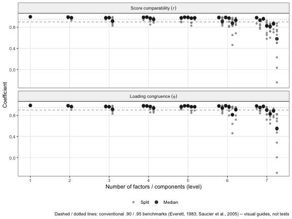

plot of chunk comparability-plot

Two honesty notes. First, the conventional benchmarks marked on the plot (.90, the replication threshold of Goldberg’s lexical research program — Everett, 1983; Saucier et al., 2005 — and .95, the stricter bound at which factors are conventionally treated as interchangeable) are conventions, not tests — comparability() reports every coefficient and flags nothing, so borderline cases stay visible and the judgment stays yours. Second, comparability is internal replication: it asks whether the structure re-emerges in halves of the same sample. That is the right gate for “is this factor real here,” and a necessary condition for — but not a demonstration of — replication in a new population.

The result is a hierarchy floor: the deepest level at which every factor replicates. For these data that is k = 5 — the Big Five, as it should be.

Step 3: Fit the hierarchy to the gated depth

x <- ackwards(bfi, k_max = 5)
print(x)
#> 
#> ── Bass-Ackwards Analysis (ackwards) ───────────────────────────────────────────
#> Engine: pca
#> Rotation: varimax
#> Basis: pearson
#> n: 875
#> k (max): 5
#> 
#> ── Levels ──
#> 
#> ✔ k = 1: 1 factor, 20.9% variance
#> ✔ k = 2: 2 factors, 32.3% variance
#> ✔ k = 3: 3 factors, 40.7% variance
#> ✔ k = 4: 4 factors, 47.8% variance
#> ✔ k = 5: 5 factors, 53.8% variance
#> 
#> ── Edges ──
#> 
#> 14 of 40 edges have |r| ≥ 0.3
#> ────────────────────────────────────────────────────────────────────────────────
#> Note: This is a series of linked solutions, not a fitted hierarchical model.
#> Cross-level edges are descriptive score correlations. Per-level fit indices
#> (EFA/ESEM) describe how well a k-factor model fits the items at that level --
#> they do not validate the edges or the hierarchy itself.

autoplot(x)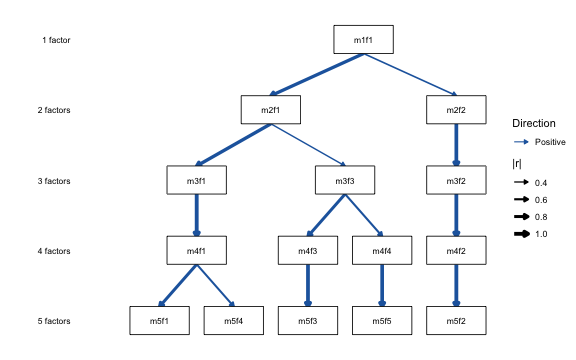

plot of chunk hierarchy-plot

If you prefer to display the fragmentation beyond the floor (it can be substantively interesting to show a factor dissolving), fit one level deeper and say explicitly in your report which levels passed the replicability gate. What the gate rules out is interpreting the deeper factors as constructs.

Step 4: Find what perpetuates without differentiating — `prune()`

Replicability is necessary but not sufficient: a factor can re-emerge in every half-sample and still add nothing, because it is the same construct restated level after level. That is Forbes’s (2023) redundancy question, and it is prune()’s job, not comparability()’s:

pr <- prune(x, "redundant")
#> ℹ Redundancy pruning (direct criterion, |r| ≥ 0.9) flagged 6 nodes.
#> ℹ Nodes are retained in the object; inspect with `x$prune$nodes` and
#>   `x$prune$chains`.
pr$prune$chains
#>    chain_id   id level r_to_prev phi_to_prev retain endpoint_r
#> 1         1 m2f2     2        NA          NA  FALSE  0.9648941
#> 2         1 m3f2     3 0.9703055   0.9780829  FALSE  0.9648941
#> 3         1 m4f2     4 0.9853622   0.9916584  FALSE  0.9648941
#> 4         1 m5f2     5 0.9990140   0.9995122   TRUE  0.9648941
#> 5         2 m3f1     3        NA          NA   TRUE  0.9978857
#> 6         2 m4f1     4 0.9978857   0.9988054  FALSE  0.9978857
#> 7         3 m4f3     4        NA          NA  FALSE  0.9773027
#> 8         3 m5f3     5 0.9773027   0.9872943   TRUE  0.9773027
#> 9         4 m4f4     4        NA          NA  FALSE  0.9570776
#> 10        4 m5f5     5 0.9570776   0.9671856   TRUE  0.9570776
#>    endpoint_r_agrees
#> 1               TRUE
#> 2               TRUE
#> 3               TRUE
#> 4               TRUE
#> 5               TRUE
#> 6               TRUE
#> 7               TRUE
#> 8               TRUE
#> 9               TRUE
#> 10              TRUE

Here the chains tell us that several of the Big Five arrive early and simply persist — for example one factor emerges at k = 2 and travels essentially unchanged (r ≥ .97 at every link) down to k = 5. Every node on that chain replicates beautifully; the chain flags that the intermediate appearances add no resolution. The two verbs answer different questions, and reporting both gives the honest picture: which levels are real, and which levels are new. See vignette("ackwards-forbes") for chain mechanics, thresholds, and the retention rule.

How sure are we about these edges? `boot_edges()`

prune()’s redundancy rule and the Forbes practice of reading off the strongest skip-level correlation both consume a point estimate at a hard threshold, so the natural follow-up is how precisely each edge is estimated. boot_edges() attaches a nonparametric bootstrap standard error and percentile confidence interval to every edge. Each replicate resamples respondents, recomputes the correlations, refits the whole hierarchy, and — importantly — re-anchors each replicate’s factors to the full-sample solution (the same matching and sign-orientation comparability() uses), so factor label-switching across replicates does not contaminate the intervals. It runs on the PCA and EFA engines with a Pearson or Spearman basis — a polychoric matrix is too slow and unstable to re-estimate in every replicate (the same scope as comparability()), so screen edge stability on the Pearson basis even when the final model is polychoric.

x_boot <- ackwards(bfi, k_max = 5, pairs = "all") |>
  boot_edges(bfi, n_boot = 200, seed = 1)
#> ℹ Fitting 200 bootstrap replicates (pca, k = 1-5)...
#> ✔ Fitting 200 bootstrap replicates (pca, k = 1-5)... [3.6s]
#> 

boot_tbl <- tidy(x_boot, what = "edges", sort = "strength")
skip_boot <- boot_tbl[
  abs(boot_tbl$level_to - boot_tbl$level_from) > 1 & abs(boot_tbl$r) >= 0.5,
  c("from", "to", "r", "lo", "hi")
]
head(skip_boot, 6)
#>    from   to         r        lo        hi
#> 4  m3f2 m5f2 0.9852300 0.9541520 0.9984825
#> 7  m2f2 m4f2 0.9673808 0.8942028 0.9916158
#> 8  m2f2 m5f2 0.9648941 0.8883935 0.9893501
#> 12 m2f1 m4f1 0.8700141 0.7593997 0.9290617
#> 14 m3f3 m5f3 0.8084301 0.5312592 0.9636492
#> 15 m3f1 m5f1 0.8080606 0.6585810 0.9044025

The lo/hi columns are the 95% percentile interval. A skip-level edge whose interval sits comfortably above prune()’s redundancy_r threshold (0.9 by default) is a defensible “same construct” claim; one whose interval straddles the threshold should not be treated as decisively redundant. The intervals are per-edge error bars, not a familywise guarantee: they do not correct for having searched the full edge table for the largest value, so a strongest-edge claim should still be pre-specified rather than selected after the fact.

Step 5: Interpret with the built-in guardrails

top_items(x, level = 5, cut = 0.5)
#> 
#> ── Salient items by factor (ackwards) ──────────────────────────────────────────
#> Engine: pca
#> Cut: |loading| >= 0.5
#> Top-n: all
#> 
#> ── Level 5 (5 factors) ──
#> 
#> m5f1
#> E2 [-0.720]
#> E4 [0.704]
#> E1 [-0.685]
#> E3 [0.659]
#> E5 [0.584]
#> 
#> m5f2
#> N3 [-0.799]
#> N1 [-0.787]
#> N2 [-0.782]
#> N5 [-0.656]
#> N4 [-0.626]
#> 
#> m5f3
#> C2 [0.702]
#> C4 [-0.692]
#> C1 [0.671]
#> C3 [0.653]
#> C5 [-0.627]
#> 
#> m5f4
#> A3 [0.698]
#> A2 [0.672]
#> A1 [-0.672]
#> A5 [0.569]
#> A4 [0.513]
#> 
#> m5f5
#> O5 [-0.676]
#> O3 [0.617]
#> O2 [-0.586]
#> O1 [0.554]
#> ────────────────────────────────────────────────────────────────────────────────
#> Loadings reflect primary-parent sign alignment. Use tidy(x, what = "loadings")
#> for the full matrix.

Three interpretation habits keep the analysis honest (all covered in depth in vignette("ackwards-interpret")):

Negative loadings do not mean “low” — sign is anchored to the primary parent, and a negative secondary edge is information, not error.
Name factors within levels, borrowing names down the lineage rather than treating each level as a fresh exploratory result.
Say what the hierarchy is. A bass-ackwards result is a series of linked solutions whose edges are score correlations — it is descriptive, not a fitted hierarchical model (no Schmid–Leiman, no higher-order SEM), and should be reported as such.

Step 6: Validate downstream, out of sample

The final step closes the loop the same way it opened: with data the model has not seen. Scores for new observations use the fit-time metric, so training and test scores are directly comparable:

train <- bfi[1:600, ]
test <- bfi[601:875, ]

x_train <- ackwards(train, k_max = 5)
test_scores <- predict(x_train, newdata = test)
round(head(test_scores[, grep("^\\.m5", names(test_scores))], 3), 2)
#>   .m5f1 .m5f2 .m5f3 .m5f4 .m5f5
#> 1  0.21 -2.77 -1.21 -1.45 -0.27
#> 2  0.19 -1.20  0.28 -1.21 -1.41
#> 3 -0.91 -1.46  1.34  0.06 -0.98

If a downstream claim (a correlation with an outcome, a group difference) holds for training-sample scores but not test-sample scores, the hierarchy was fine and the claim was overfit — a different failure than anything in Steps 1–5, and one only held-out data can catch. The train/test mechanics are covered in vignette("ackwards-intro").

Common mistakes this workflow prevents

Interpreting non-replicable deep factors. The classic failure. Without a replicability instrument the deep levels are just there, printed with the same authority as the robust ones. Step 2 makes their status measurable and visible.

Trusting a single split. One split-half can flatter or slander a factor by luck of the draw. comparability() defaults to ten random splits and reports the spread; the minima across splits are as informative as the medians.

Cherry-picking the strongest edge. With pairs = "all", the number of between-level correlations grows fast, and reporting the most dramatic one capitalizes on chance. Report full edge tables (or the complete diagram), and treat any “strongest link” claim as descriptive rather than inferential. boot_edges() (Step 4 above) attaches a bootstrap confidence interval to every edge, which makes each estimate’s precision visible — useful for judging whether an edge clears prune()’s redundancy threshold — but per-edge intervals do not undo the selection bias of scanning many edges for the largest.

Mistaking persistence for structure. A chain of near-1.0 correlations down the hierarchy looks impressive but means the levels are restating one construct. That is a prune() finding, and it should shorten your reported k range, not lengthen your list of constructs.

Mistaking replicability for validity. A comparability of .99 means the factor is a stable feature of these items in this population — not that it is a good construct, and not that it generalizes beyond the population sampled. Cross-population replication and external validation remain separate, subsequent steps.

Summary: the workflow in six calls

suggest_k(data) — screen the plausible depth range; treat its top as a ceiling to probe.
comparability(data, k_max = ceiling + 1) — find the hierarchy floor: the deepest level at which every factor replicates across split-halves.
ackwards(data, k_max = floor) — fit the hierarchy to the gated depth.
prune(x, "redundant") — identify factors that perpetuate without differentiating; report which levels add resolution.
top_items(x) + autoplot(x) — interpret with the sign, naming, and descriptive-hierarchy guardrails.
predict(x_train, newdata = test) — validate downstream claims on held-out data in the fit-time metric.

Steps 1, 3, 4, and 5 are the established method. Step 2 restores the gate the method’s own inventor applied to it, and Step 6 extends the same logic — show me it holds in data you did not fit — to whatever you do with the scores.

References

Everett, J. E. (1983). Factor comparability as a means of determining the number of factors and their rotation. Multivariate Behavioral Research, 18(2), 197–218. https://doi.org/10.1207/s15327906mbr1802_5

Forbes, M. K. (2023). Improving hierarchical models of individual differences: An extension of Goldberg’s bass-ackward method. Psychological Methods. https://doi.org/10.1037/met0000546

Goldberg, L. R. (2006). Doing it all Bass-Ackwards: The development of hierarchical factor structures from the top down. Journal of Research in Personality, 40(4), 347–358. https://doi.org/10.1016/j.jrp.2006.01.001

Lorenzo-Seva, U., & ten Berge, J. M. F. (2006). Tucker’s congruence coefficient as a meaningful index of factor similarity. Methodology, 2(2), 57–64. https://doi.org/10.1027/1614-2241.2.2.57

Saucier, G. (1997). Effects of variable selection on the factor structure of person descriptors. Journal of Personality and Social Psychology, 73(6), 1296–1312. https://doi.org/10.1037/0022-3514.73.6.1296

Saucier, G., Georgiades, S., Tsaousis, I., & Goldberg, L. R. (2005). The factor structure of Greek personality adjectives. Journal of Personality and Social Psychology, 88(5), 856–875. https://doi.org/10.1037/0022-3514.88.5.856