Ordinal Data: Polychoric Correlations and WLSMV

Most psychological scales use ordinal response formats: Likert-type items with a handful of ordered categories, binary (yes/no) items, and everything in between. Treating these as continuous and computing Pearson correlations between them is ubiquitous in practice, but it introduces systematic bias that can distort both loadings and the between-level edges that bass-ackwards analysis depends on. This vignette explains the problem and how ackwards addresses it.

Why Pearson underestimates for ordinal items

When a continuous latent trait is sliced into a small number of ordered categories, the observed correlation between two items is always lower than the correlation between their underlying latent variables. The more coarse the rating scale, the larger the attenuation. For a 5-point scale, Pearson correlations can be 10–20% lower than the true latent correlations; for a 2-point (binary) scale, the underestimate can exceed 30%.

This matters for bass-ackwards analysis because:

1. Loadings are attenuated. Factors appear weaker than they are.
2. Between-level edges are attenuated. The hierarchy looks flatter — factors that should be nearly perfectly correlated across levels may appear only moderately correlated.
3. The number of factors is underestimated. Attenuation compresses the eigenvalue spectrum, so selection criteria (parallel analysis, MAP) may suggest fewer factors than truly exist.

The polychoric solution

A polychoric correlation between two ordinal items estimates the Pearson correlation that would exist between their underlying continuous latent variables, if those variables had been measured without discretization. It does this by fitting a bivariate normal model with thresholds at each category boundary.

For binary (two-category) items this same estimate is traditionally called a tetrachoric correlation, but it is not a separate method — tetrachoric is simply the two-category special case of polychoric. cor = "polychoric" handles binary items automatically: psych::polychoric() detects the two-level case and returns the tetrachoric estimate, so you never request tetrachoric separately.

Setting cor = "polychoric" in ackwards() replaces step 1 of the pipeline — computing the item correlation matrix R — with a polychoric matrix. All downstream computation (factor extraction, rotation, tenBerge scoring, between-level algebra) then operates on that polychoric R.

Automatic detection

ackwards() checks for ordinal-looking data using a simple heuristic: if any column is integer-valued with ≤ 7 distinct levels, the data is flagged and a warning is issued when cor = "pearson" (the default).

library(ackwards)
bfi <- na.omit(bfi25)

# The warning fires with the default Pearson basis
x_pearson <- ackwards(bfi, k_max = 5)

The warning is ackwards reminding you to make an active choice. Specifying cor = "polychoric" acknowledges the data type and suppresses it:

x_poly <- ackwards(bfi, k_max = 5, cor = "polychoric")

Seeing the difference

Correlation matrices

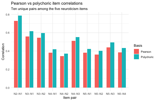
The most direct way to see the impact of the basis is to compare the item correlations under each basis. Rather than read two 5×5 matrices side by side, the chart below plots the ten unique item-pair correlations among the five neuroticism items (N1–N5), Pearson against polychoric.

plot of chunk r-compare

Every polychoric bar sits above its Pearson counterpart — the correlations are consistently higher. The N1–N2 pair, for instance, goes from about 0.73 (Pearson) to 0.79 (polychoric); across the block the increase runs to roughly 0.05, enough to shift loadings and change eigenvalues.

Loadings

The table below compares primary loadings — the loading of each Neuroticism item on its dominant factor — under both correlation bases at k = 5. The Δ column is the attenuation: how much larger each loading becomes (in absolute value) once the polychoric basis removes the coarse-category suppression. Using |Polychoric| − |Pearson| keeps the attenuation positive regardless of loading sign.

Neuroticism-item loadings at k = 5: Pearson vs polychoric
Positive Δ = attenuation removed by the polychoric basis
Item	Factor	Primary loading
		Pearson	Polychoric	Δ (|Poly| − |Pearson|)1
N1	m5f2	−0.79	−0.81	0.02
N2	m5f2	−0.78	−0.81	0.02
N3	m5f2	−0.80	−0.82	0.03
N4	m5f2	−0.63	−0.65	0.02
N5	m5f2	−0.66	−0.69	0.03
1 Factor assignment and sign verified to match between bases. Delta uses |Poly| - |Pearson| so attenuation is positive regardless of loading sign.

Polychoric loadings for the Neuroticism items are noticeably higher — the latent structure is sharper when the attenuating effect of coarse categories is removed.

Between-level edges

The same comparison for the primary-parent edges. The Δ column is the change in connection strength (|r|): positive where the polychoric basis recovers a stronger connection by undoing attenuation, negative in the few cases where the recovered structure is slightly looser. Using absolute values makes the direction read correctly even for the negatively-signed edge.

Primary-parent edges: Pearson vs polychoric
Δ = change in |r|; positive = stronger connection under polychoric basis
From	To	Edge strength (r)
		Pearson	Polychoric	Δ (|Poly| − |Pearson|)1
m1f1	m2f1	0.88	0.89	0.01
m1f1	m2f2	0.48	0.46	−0.02
m2f1	m3f1	0.90	0.87	−0.02
m2f2	m3f2	0.97	0.99	0.02
m2f1	m3f3	0.43	0.48	0.05
m3f1	m4f1	1.00	0.99	0.00
m3f2	m4f2	0.99	0.98	−0.01
m3f3	m4f3	0.80	0.73	−0.07
m3f3	m4f4	0.59	0.68	0.09
m4f1	m5f1	0.82	0.84	0.02
m4f2	m5f2	1.00	1.00	0.00
m4f3	m5f3	0.98	0.98	0.01
m4f1	m5f4	0.58	0.55	−0.03
m4f4	m5f5	0.96	0.99	0.03
1 NA in either column means the bases disagree on the primary parent for that factor.

The edges are broadly similar in sign and rank order — the hierarchy is the same — but polychoric edges are stronger. Factors that represent genuinely stable dimensions show near-perfect correlations with their counterparts at adjacent levels when the true latent structure is properly recovered.

WLSMV for ESEM with ordinal items

When engine = "esem" and cor = "polychoric" are combined, ackwards() automatically switches the lavaan estimator to WLSMV (diagonally weighted least squares, mean- and variance-adjusted). This is the standard estimator for structural equation models with categorical or ordinal indicators, and is the same method used by Mplus by default.

WLSMV genuinely operates on the polychoric basis: lavaan estimates the item thresholds and the polychoric correlations among the ordinal indicators, then fits the factor model to that matrix using a diagonal weight matrix. So combining cor = "polychoric" with the ESEM engine is not stacking two separate corrections — the polychoric structure is precisely what WLSMV is built to model, and the between-level edges are computed from lavaan’s own latent correlation matrix (not a separately estimated psych polychoric matrix).

x_esem <- ackwards(bfi, k_max = 3, engine = "esem", cor = "polychoric")
x_esem
#> 
#> ── Bass-Ackwards Analysis (ackwards) ───────────────────────────────────────────
#> Engine: esem
#> Rotation: varimax
#> Basis: polychoric
#> n: 875
#> k (max): 3
#> 
#> ── Levels ──
#> 
#> ✔ k = 1: 1 factor, 23.5% variance
#> ✔ k = 2: 2 factors, 32.9% variance
#> ✔ k = 3: 3 factors, 39.5% variance
#> 
#> ── Edges ──
#> 
#> 5 of 8 edges have |r| ≥ 0.3
#> ────────────────────────────────────────────────────────────────────────────────
#> Note: This is a series of linked solutions, not a fitted hierarchical model.
#> Cross-level edges are descriptive score correlations. Per-level fit indices
#> (EFA/ESEM) describe how well a k-factor model fits the items at that level --
#> they do not validate the edges or the hierarchy itself.

The WLSMV fit indices (CFI, RMSEA, SRMR) are now computed on a model that respects the ordinal measurement level. They will typically look better than Pearson-based fit indices on the same data, reflecting both the better model specification and the different reference distribution WLSMV uses.

tidy(x_esem, what = "fit", format = "wide")
#>   level      chi dof p_value       CFI       TLI     RMSEA       SRMR BIC
#> 1     2 3616.834 251       0 0.7117569 0.6554864 0.1238665 0.09547997  NA
#> 2     3 2448.356 228       0 0.8098533 0.7498069 0.1055573 0.07172502  NA

See vignette("ackwards-engines"), section “Per-level fit: what it tells you (and what it doesn’t)”, for how to interpret these indices in the bass-ackwards context and how to produce the autoplot(what = "fit") trajectory chart.

Practical guidance: when to use polychoric

Scale characteristics	Recommendation
Continuous or many categories (> 7)	cor = "pearson" (default)
5–7 ordered categories (typical Likert)	cor = "polychoric" — recommended
3–4 categories	cor = "polychoric" — strongly recommended
Binary (2 categories)	cor = "polychoric" — essential (this is the tetrachoric case)

Polychoric estimation requires fitting a bivariate normal model for every item pair. With p items that is p(p−1)/2 pairs — about 300 for a 25-item scale. Computation is usually fast (seconds), but scales as O(p²) and can be slow for very large item pools.

Screen skewed or sparse scales first. Clinical symptom scales and other right-skewed items often have a response category endorsed by only a handful of people. That can make psych::polychoric() fail under its default continuity correction (set correct = 0), and — with many such items — drive the correlation matrix near-singular, in which case per-level fit indices (especially CFI, which comes back NA) and factor scores become unreliable. Run [check_items()][ackwards::check_items] before fitting to see which items are degenerate or sparse, and read the “When to trust the result” section of ?ackwards for how each warning maps to whether you should report the solution. When a matrix is near-singular, ackwards() says so once and records it on the object, so print()/summary() keep reminding you.

[factorability()][ackwards::factorability] is the companion screen for the correlation matrix as a whole: it reports the KMO measure of sampling adequacy (overall and per item), Bartlett’s test of sphericity, the N:p ratio, and the Ledermann bound on how many factors p items can identify. Call it on the same cor basis you plan to fit. Read its output as conventions, not verdicts — the KMO bands and N:p rules of thumb are contested — but a very low KMO or a handful of low-MSA items is a useful early signal. ackwards() runs a light version of this screen internally and warns only at the consequential extreme (KMO below .5, N:p below 5, or k_max past the Ledermann bound for EFA/ESEM).

A note on score computation. The short answer: yes, you can use the factor scores from an ordinal analysis in downstream work — the caveat below is about scaling, not validity. When cor = "polychoric", the weight matrices stored in the object are derived from the polychoric R, but augment() materializes scores by applying those weights to Pearson-standardized raw data (.standardize(data)). The resulting scores are calibrated to model-implied unit variance rather than exactly empirical unit variance, so their empirical standard deviations will be close to but not precisely 1. That scaling nuance is the only reason augment() warns when cor != "pearson"; the warning does not mean the scores are biased or unusable. The between-level edges from tidy(what = "edges") are unaffected either way — they come from the exact algebra, not from materialized scores.

References

Flora, D. B., & Curran, P. J. (2004). An empirical evaluation of alternative methods of estimation for confirmatory factor analysis with ordinal data. Psychological Methods, 9(4), 466–491.

Muthén, B. O. (1984). A general structural equation model with dichotomous, ordered categorical, and continuous latent variable indicators. Psychometrika, 49(1), 115–132.

Olsson, U. (1979). Maximum likelihood estimation of the polychoric correlation coefficient. Psychometrika, 44(4), 443–460.

Pearson, K. (1900). Mathematical contributions to the theory of evolution. VII. On the correlation of characters not quantitatively measurable. Philosophical Transactions of the Royal Society of London, Series A, 195, 1–47.