
Reproducing Forbes (2023): The AMH Applied Example
Source:vignettes/ackwards-forbes2023.Rmd
ackwards-forbes2023.RmdForbes (2023) introduced the extended bass-ackwards method: all-pairs between-level correlations plus redundancy pruning. A factor is an unobserved dimension that explains why a set of items correlate. A redundant factor restates a factor at another level rather than refining it. She demonstrated the method on a real, deep hierarchy: the Assessing Mental Health (AMH) study. That study measured 155 mental-health symptom variables spanning 18 DSM disorders in an Australian general-population sample (N = 3,175, Forbes et al., 2021). Her paper cites this package as the reference implementation of the extension.
The Spearman correlation matrix from that applied example ships with
the package as the forbes2023 dataset (redistributed from
Forbes’s OSF project under CC-BY 4.0, see ?forbes2023).
This vignette reproduces her published analysis end-to-end: the 10-level
hierarchy, the skip-level correlations, the redundancy chase, and the
pruned-factor diagram.
If the concepts here are new (what skip-level edges are, how
prune() decides what to flag), read
vignette("ackwards-forbes") first. It teaches the method
extension on a small didactic dataset. This vignette runs the real
thing.
The data
forbes2023 is a 155 × 155 Spearman correlation matrix,
not raw data:
library(ackwards)
dim(forbes2023)
#> [1] 155 155
forbes2023[1:3, 1:3]
#>                        Impulsivity Reckless_behaviour__i_  Blurting
#> Impulsivity              1.0000000              0.5415115 0.6172762
#> Reckless_behaviour__i_   0.5415115              1.0000000 0.4783731
#> Blurting                 0.6172762              0.4783731 1.0000000
A correlation matrix carries no sample size, so we supply the AMH
study’s N explicitly with n_obs = 3175. For the PCA engine
used here nothing downstream depends on N. PCA (principal component
analysis) summarizes the items with weighted sums called components.
Supplying N is still good practice: it is recorded in the object, and it
enables N-dependent fit statistics under the factor engines.
Fitting the 10-level hierarchy
Forbes’s applied example extracts 1 through 10 components with all between-level pairs:
x <- ackwards(forbes2023, k_max = 10, pairs = "all", n_obs = 3175)
x
#>
#> ── Bass-Ackwards Analysis (ackwards) ───────────────────────────────────────────
#> Engine: pca
#> Rotation: varimax
#> Basis: (user-supplied matrix)
#> n: 3,175
#> k (max): 10
#>
#> ── Levels ──
#>
#> ✔ k = 1: 1 factor, 31.4% variance
#> ✔ k = 2: 2 factors, 36.8% variance
#> ✔ k = 3: 3 factors, 41.1% variance
#> ✔ k = 4: 4 factors, 44.9% variance
#> ✔ k = 5: 5 factors, 48.2% variance
#> ✔ k = 6: 6 factors, 50.8% variance
#> ✔ k = 7: 7 factors, 52.9% variance
#> ✔ k = 8: 8 factors, 54.6% variance
#> ✔ k = 9: 9 factors, 56.2% variance
#> ✔ k = 10: 10 factors, 57.6% variance
#>
#> ── Edges ──
#>
#> 312 of 1320 edges have |r| ≥ 0.3
#> ────────────────────────────────────────────────────────────────────────────────
#> Note: This is a series of linked solutions, not a fitted hierarchical model.
#> Cross-level edges are descriptive score correlations. Per-level fit indices
#> (EFA/ESEM) describe how well a k-factor model fits the items at that level --
#> they do not validate the edges or the hierarchy itself.
The hierarchy unfolds a general factor of psychopathology at the top
(k = 1, ~31% of variance) down to ten fine-grained components
(cumulatively ~58%). With pairs = "all", the edge table
holds 1320 correlations across all 45 level pairs. Every one of them is
matched against Forbes’s own reference implementation by the package
regression test (see Fidelity, below).
Label mapping. Forbes labels components by level
letter and position within the level. Her a1 is the single
component at k = 1, b1 and b2 sit at k = 2,
and j1 through j10 sit at k = 10. This package
uses m{k}f{j} for the same positions, so her
d4 is m4f4 and her j4 is
m10f4. Signs may differ component by component, because the
package aligns each factor to its primary parent (see
vignette("ackwards-intro")). That leaves every correlation
identical in absolute value.
Skip-level structure
The deep hierarchy is where skip-level correlations earn their keep. Among the non-adjacent pairs alone, 48 correlations exceed |r| = 0.9. These are components that persist almost unchanged across two or more levels:
| Strongest skip-level edges in the AMH hierarchy | ||||
| Top 10 non-adjacent pairs by |r| | ||||
| From | To | Level (from) | Level (to) | r |
|---|---|---|---|---|
| m6f6 | m8f7 | 6 | 8 | 1.000 |
| m7f6 | m9f5 | 7 | 9 | 0.999 |
| m6f6 | m9f5 | 6 | 9 | 0.998 |
| m5f5 | m8f7 | 5 | 8 | 0.998 |
| m5f5 | m7f6 | 5 | 7 | 0.998 |
| m8f7 | m10f5 | 8 | 10 | 0.998 |
| m7f6 | m10f5 | 7 | 10 | 0.998 |
| m6f6 | m10f5 | 6 | 10 | 0.997 |
| m5f5 | m9f5 | 5 | 9 | 0.996 |
| m7f5 | m9f4 | 7 | 9 | 0.996 |
Correlations this close to 1.0 across multiple levels are the signature of redundancy: the intermediate solutions are relabeling a stable dimension, not refining it. That is exactly what the redundancy chase formalizes.
The redundancy chase
Forbes’s ChaseCorrPaths() procedure walks each component
upward through the hierarchy. At every ancestor level it takes the
component with the largest direct (skip-level)
correlation, and it continues while |r| ≥ 0.9. Chains of near-identical
components are then collapsed to a single retained node.
prune(x, "redundant") implements the same rule as its
default (redundancy_criterion = "direct"):
xp <- prune(x, "redundant")
#> ℹ Redundancy pruning (direct criterion, |r| ≥ 0.9) flagged 37 nodes.
#> ℹ Nodes are retained in the object; inspect with `x$prune$nodes` and
#>   `x$prune$chains`.
Of the 55 components in the full hierarchy, 37 are flagged as
redundant, leaving 18 distinct constructs. That is the same
decomposition reported in Forbes (2023). As always, prune()
only annotates. Nothing is removed from the object, and every
flagged component keeps its loadings (a loading is the correlation
between an item and a factor), scores, and edges.
A chain, worked
Forbes’s chase traces the chain
d4 → e4 → f5 → g5 → h5 → i4 → j4: one dimension surfacing
at k = 4 and persisting, near-unchanged, to k = 10. In
ackwards labels, that chain is:
ch <- xp$prune$chains
d4 <- ch[ch$chain_id == ch$chain_id[ch$id == "m10f4"], c("id", "level", "retain")]
d4
#>       id level retain
#> 14  m4f4     4  FALSE
#> 15  m5f4     5  FALSE
#> 16  m6f5     6  FALSE
#> 17  m7f5     7  FALSE
#> 18  m8f5     8  FALSE
#> 19  m9f4     9  FALSE
#> 20 m10f4    10   TRUE
Because the chain reaches the deepest level, the retention rule keeps
its bottom node, m10f4 (her
j4), the most specific and best-defined manifestation. The
rule flags the six components above it as redundant. A chain that stops
short of k = 10 instead keeps its top node, the broadest
manifestation.
The full retained set (13 chain-retained components, in level order): m1f1, m4f2, m5f2, m7f7, m10f1, m10f2, m10f3, m10f4, m10f5, m10f6, m10f7, m10f8, m10f9. The other 5 kept components were never part of a |r| ≥ 0.9 chain at all, so no retention rule applies to them.
Why the direct criterion matters here
Correlation is not transitive: a chain of adjacent links each ≥ 0.9 does not guarantee the two ends correlate ≥ 0.9 directly. On shallow hierarchies the distinction rarely bites, but on this 10-level hierarchy it does. Forbes’s direct rule and an adjacent-hop walk disagree on 7 of the 54 chased components:
xa <- prune(x, "redundant", redundancy_criterion = "adjacent")
#> ℹ Redundancy pruning (adjacent criterion, |r| ≥ 0.9) flagged 36 nodes.
#> ℹ Nodes are retained in the object; inspect with `x$prune$nodes` and
#>   `x$prune$chains`.
The adjacent opt-in flags 36 components (vs 37 under the default) and
retains m3f3, which the direct rule chases further up the
hierarchy. The default reproduces Forbes’s published chase exactly, all
54 components, including those 7 divergences. So stick with it when your
goal is comparability with her method.
redundancy_criterion = "adjacent" remains available for
sensitivity analysis.
The pruned-factor diagram
Dropping the flagged components and bridging each retained component directly to its strongest kept ancestor yields the pruned-factor diagram. It uses the same publication style as Forbes (2023): black lines, uniform width, no legend, and correlation labels on each spanning arrow.
autoplot(xp,
  drop_pruned = TRUE, show_r = TRUE,
  color_pos = "black", color_neg = "black",
  edge_linewidth = 0.6, show_arrows = FALSE, legend = FALSE
)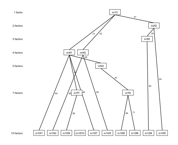
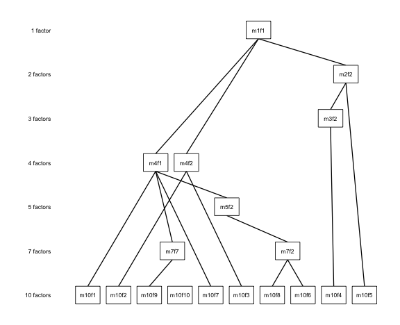
Whole levels vanish (every component at those levels was flagged), leaving deliberate gaps in the y-axis. To compact the layout while keeping the original level numbers:
autoplot(xp,
  drop_pruned = TRUE, compress_levels = TRUE,
  color_pos = "black", color_neg = "black",
  edge_linewidth = 0.6, show_arrows = FALSE, legend = FALSE
)
For the full set of cosmetic controls, see
vignette("ackwards-visualization").
Fidelity
This reproduction is not merely visual. It is pinned by the package’s
regression suite (tests/testthat/test-forbes-fidelity.R),
which verifies on every check run that:
- all 45 between-level correlation matrices match the output of Forbes’s own reference implementation entrywise in absolute value (tolerance 1e-12), and
- the direct redundancy chase lands on her published
ChaseCorrPaths()result for all 54 chased components.
The expected values were computed with Forbes’s reference
implementation (from her OSF project,
https://osf.io/pcwm8/) on the same md5-pinned matrix that
ships as forbes2023. So the dataset and the oracle cannot
drift apart. Only ackwards() runs at test time.
References
Forbes, M. K. (2023). Improving hierarchical models of individual differences: An extension of Goldberg’s bass-ackward method. Psychological Methods. https://doi.org/10.1037/met0000546
Forbes, M. K., Sunderland, M., Rapee, R. M., Batterham, P. J., Calear, A. L., Carragher, N., Ruggero, C., Zimmerman, M., Baillie, A. J., Lynch, S. J., Mewton, L., Slade, T., & Krueger, R. F. (2021). A detailed hierarchical model of psychopathology: From individual symptoms up to the general factor of psychopathology. Clinical Psychological Science, 9(2), 139–168. https://doi.org/10.1177/2167702620954799
Goldberg, L. R. (2006). Doing it all Bass-Ackwards: The development of hierarchical factor structures from the top down. Journal of Research in Personality, 40(4), 347–358. https://doi.org/10.1016/j.jrp.2006.01.001