
ackwards supports three factor extraction engines. A
factor is an unobserved dimension that explains why a set of items
correlate. The engines share the same downstream machinery: the same
default rotation, correlation-preserving scoring weights, and the same
W′RW between-level correlation algebra. The weights are ten
Berge weights for EFA and ESEM and component score weights for PCA. A
rotation re-orients the factors within a level without changing how well
they fit. The engines differ in their statistical model and in what they
report. This vignette explains when each one is appropriate and what the
differences look like in practice.
The three engines at a glance
A few terms recur in the table below. PCA (principal component analysis) summarizes the items with weighted sums called components. EFA (exploratory factor analysis) models the items as a small number of shared factors plus item-specific noise. ESEM (exploratory structural equation modeling) fits that same factor model in lavaan and adds standard errors. A polychoric correlation estimates the correlation between two ordinal items, items recorded on an ordered scale with few categories, as if each were a continuous variable cut into categories. FIML (full-information maximum likelihood) uses every partially observed row of the data instead of dropping it. A loading is the correlation between an item and a factor under the default varimax rotation. Under an oblique rotation it is the item’s regression weight on the factor.
"pca" |
"efa" |
"esem" |
|
|---|---|---|---|
| What it models | Total item variance | Common (latent) variance | Common (latent) variance |
| Engine substrate | psych::principal() |
psych::fa() |
lavaan |
| Communalities | All 1.0 (by definition) | Estimated from data | Estimated from data |
| Correlations | Pearson or polychoric | Pearson or polychoric | Pearson or polychoric |
| Estimators | Eigen-decomposition |
minres (OLS), ml, or pa, via
psych’s fm=
|
ML or MLR for continuous data (plus FIML for missing data). WLSMV or ULSMV for ordinal data |
| Fit indices | Eigenvalues only | χ², RMSEA, TLI, BIC | CFI, TLI, RMSEA, SRMR, χ² |
| Loading SEs | No | No | Yes |
| Speed | Fast | Moderate | Slowest |
| Best for | Exploration, large k | Latent-factor inference | Model evaluation, loading SEs, ordinal or continuous |
All three produce the same labels (m{k}f{j}), the same
tidy() / glance() / augment()
interface, and comparable between-level edges for well-structured data.
The hierarchy they reveal is usually the same. The statistical
guarantees differ.
Setup
We use the BFI-25 with polychoric correlations throughout, so that differences in output reflect the engine and not the correlation basis.
PCA: components from total variance
PCA extracts principal components, linear combinations of the observed variables that capture maximum variance, including measurement error. Every item is modeled with communality 1.0: the components account for 100% of each item’s variance. This is not a true latent variable model. It is a data reduction method.
In the bass-ackwards context, PCA is the natural default. It is fast,
always converges, and produces eigenvalues that can guide the choice of
k. Waller (2007) showed that, for components, the correlations between
the scores of two levels follow from the transformation matrices that
rotate each level’s components, with no scores computed. The
W′RW algebra gives the same correlations from the component
weights. The edges are exact for the correlation matrix the fit uses.
That matrix is polychoric here, so scores computed from the observed
items do not in general reproduce the edges. The same is true when the
matrix is Spearman, or when it is estimated from incomplete data by
pairwise deletion or by FIML. Pairwise deletion computes each
correlation from only the rows where both items are observed.
x_pca <- ackwards(bfi, k_max = 3, cor = "polychoric")
x_pca
#>
#> ── Bass-Ackwards Analysis (ackwards) ───────────────────────────────────────────
#> Engine: pca
#> Rotation: varimax
#> Basis: polychoric
#> n: 875
#> k (max): 3
#>
#> ── Levels ──
#>
#> ✔ k = 1: 1 factor, 23.2% variance
#> ✔ k = 2: 2 factors, 35.5% variance
#> ✔ k = 3: 3 factors, 44.6% variance
#>
#> ── Edges ──
#>
#> 5 of 8 edges have |r| ≥ 0.3
#> ────────────────────────────────────────────────────────────────────────────────
#> Note: This is a series of linked solutions, not a fitted hierarchical model.
#> Cross-level edges are descriptive score correlations. Per-level fit indices
#> (EFA/ESEM) describe how well a k-factor model fits the items at that level --
#> they do not validate the edges or the hierarchy itself.
The “fit” for PCA is just the eigenvalue of each component, the amount of variance it captures. There are no chi-square tests, no RMSEA, no model rejection.
tidy(x_pca, what = "fit")
#>   level       statistic    value
#> 1     1 eigenvalue.m1f1 5.802803
#> 2     2 eigenvalue.m2f1 5.802803
#> 3     2 eigenvalue.m2f2 3.067627
#> 4     3 eigenvalue.m3f1 5.802803
#> 5     3 eigenvalue.m3f2 3.067627
#> 6     3 eigenvalue.m3f3 2.275419
EFA: factors from common variance
EFA extracts latent factors that model only the variance shared among items. Each item retains a unique variance (communality < 1.0) that the factors do not explain. This is the classical common-factor model. It is more appropriate than PCA when you believe the items are fallible indicators of latent constructs rather than the constructs themselves.
x_efa <- ackwards(bfi, k_max = 3, engine = "efa", cor = "polychoric")
x_efa
#>
#> ── Bass-Ackwards Analysis (ackwards) ───────────────────────────────────────────
#> Engine: efa
#> Rotation: varimax
#> Basis: polychoric
#> n: 875
#> k (max): 3
#>
#> ── Levels ──
#>
#> ✔ k = 1: 1 factor, 20.3% variance
#> ✔ k = 2: 2 factors, 30.8% variance
#> ✔ k = 3: 3 factors, 37.7% variance
#>
#> ── Edges ──
#>
#> 5 of 8 edges have |r| ≥ 0.3
#> ────────────────────────────────────────────────────────────────────────────────
#> Note: This is a series of linked solutions, not a fitted hierarchical model.
#> Cross-level edges are descriptive score correlations. Per-level fit indices
#> (EFA/ESEM) describe how well a k-factor model fits the items at that level --
#> they do not validate the edges or the hierarchy itself.
EFA produces genuine goodness-of-fit indices. These tell you whether the k factors are sufficient to reproduce the observed correlation matrix within sampling error.
tidy(x_efa, what = "fit")
#>    level statistic        value
#> 1      1       chi 5327.2295200
#> 2      1       dof  275.0000000
#> 3      1   p_value    0.0000000
#> 4      1     RMSEA    0.1448964
#> 5      1       TLI    0.3429279
#> 6      1       BIC 3464.3179512
#> 7      2       chi 3520.3788570
#> 8      2       dof  251.0000000
#> 9      2   p_value    0.0000000
#> 10     2     RMSEA    0.1220036
#> 11     2       TLI    0.5337688
#> 12     2       BIC 1820.0486615
#> 13     3       chi 2545.6948352
#> 14     3       dof  228.0000000
#> 15     3   p_value    0.0000000
#> 16     3     RMSEA    0.1077785
#> 17     3       TLI    0.6358514
#> 18     3       BIC 1001.1717891
The RMSEA values here are large (> 0.10). They indicate that 1 to 3 factors do not fully account for the BFI item correlations, which is no surprise, because the true structure is 5 factors. Fit improves steadily from k = 1 to k = 3. That is exactly the kind of evidence bass-ackwards analysis is designed to make visible.
How close are EFA and PCA loadings?
For clean, continuous data with moderate-to-strong factor structure, EFA and PCA loadings are highly correlated but not identical. EFA loadings are systematically somewhat smaller because they model only the common variance. PCA inflates loadings by fitting noise alongside signal.
The table below compares primary loadings, the loading of each item on its dominant factor, for six representative items at k = 3. The items are two each from the Neuroticism, Extraversion, and Conscientiousness families. The Δ column is the teaching point: how much smaller EFA loadings are in absolute value once measurement error is partitioned into uniqueness. Using |EFA| − |PCA| keeps the attenuation consistently negative regardless of loading sign.
| PCA vs EFA: primary loadings for anchor items (k = 3) | ||||
| Item | Factor |
Loading
|
||
|---|---|---|---|---|
| PCA | EFA | Δ (|EFA| − |PCA|)1 | ||
| E1 | m3f1 | −0.61 | −0.55 | −0.06 |
| E2 | m3f1 | −0.70 | −0.67 | −0.03 |
| N1 | m3f2 | −0.78 | −0.75 | −0.03 |
| N2 | m3f2 | −0.79 | −0.76 | −0.03 |
| C1 | m3f3 | 0.66 | 0.62 | −0.04 |
| C2 | m3f3 | 0.64 | 0.61 | −0.03 |
| 1 Factor assignment and sign verified to match between engines. Delta uses |EFA| - |PCA| so attenuation is always negative regardless of loading sign. | ||||
EFA loadings for the same items are consistently a few points lower. The PCA loadings include some noise variance that EFA partitions into uniqueness. The factor structure (which items define which factor) is unchanged.
ESEM: EFA with full model diagnostics
ESEM (exploratory structural equation modeling, Asparouhov & Muthén, 2009) fits the same common-factor model as EFA but uses lavaan as the engine. ESEM is not an ordinal-only tool. It handles continuous items with maximum-likelihood estimators (ML or MLR, the default for continuous data) and ordinal items with WLSMV. It unlocks three capabilities that EFA cannot provide:
- Standard errors for every loading, which enable confidence intervals and significance tests, for continuous and ordinal data.
-
Full maximum-likelihood estimation for continuous
data (ML/MLR), including FIML for missing data
(
missing = "fiml"), which uses all partially observed rows rather than deleting them. -
The WLSMV estimator for ordinal data, the
appropriate maximum-likelihood-adjacent estimator for categorical
indicators. When
cor = "polychoric"is set withengine = "esem", WLSMV is used automatically.
Those three are the only reasons to pay ESEM’s cost (a lavaan fit per level, occasional convergence trouble). EFA is otherwise a first-class reporting engine. It returns the same loadings, variance, and between-level edges plus per-level RMSEA and TLI, which is enough to report a hierarchy. Reach for ESEM when you need loading standard errors (especially at smaller n), the field-standard WLSMV estimator for ordinal indicators, or true FIML for missing data. Otherwise EFA is the simpler, faster choice.
x_esem <- ackwards(bfi, k_max = 3, engine = "esem", cor = "polychoric")
x_esem
#>
#> ── Bass-Ackwards Analysis (ackwards) ───────────────────────────────────────────
#> Engine: esem
#> Rotation: varimax
#> Basis: polychoric
#> n: 875
#> k (max): 3
#>
#> ── Levels ──
#>
#> ✔ k = 1: 1 factor, 23.5% variance
#> ✔ k = 2: 2 factors, 32.9% variance
#> ✔ k = 3: 3 factors, 39.5% variance
#>
#> ── Edges ──
#>
#> 5 of 8 edges have |r| ≥ 0.3
#> ────────────────────────────────────────────────────────────────────────────────
#> Note: This is a series of linked solutions, not a fitted hierarchical model.
#> Cross-level edges are descriptive score correlations. Per-level fit indices
#> (EFA/ESEM) describe how well a k-factor model fits the items at that level --
#> they do not validate the edges or the hierarchy itself.
ESEM fit indices include CFI and SRMR in addition to RMSEA and TLI, which gives a richer picture of model adequacy. See the “Per-level fit” section below for how to report and interpret these indices.
Loading standard errors and confidence intervals
The unique output from ESEM is the rotation-aware standard
error of every loading. These SEs are returned as part of
tidy(what = "loadings"), alongside ci_lower
and ci_upper columns:
ld <- tidy(x_esem, what = "loadings")
head(ld)
#>   level factor item    loading         se   ci_lower   ci_upper
#> 1     1   m1f1   A1 -0.3155807 0.02831633 -0.3710797 -0.2600817
#> 2     1   m1f1   A2  0.5584169 0.02316777  0.5130089  0.6038249
#> 3     1   m1f1   A3  0.6424786 0.01971862  0.6038308  0.6811264
#> 4     1   m1f1   A4  0.4261675 0.02777029  0.3717387  0.4805962
#> 5     1   m1f1   A5  0.6588505 0.01870826  0.6221830  0.6955180
#> 6     1   m1f1   C1  0.4138252 0.02754885  0.3598304  0.4678200
The intervals are computed as loading ± z × SE (default
95%). Set conf_level = 0.99 for wider intervals. With the
875 complete cases used here the SEs are fairly small. With smaller
samples they become important for judging which loadings are
meaningfully non-zero. For PCA and EFA objects the se,
ci_lower, and ci_upper columns are present but
NA, because those engines carry no loading SEs.
Per-level fit: what it tells you (and what it does not)
The key distinction
Bass-ackwards produces a series of independent factor solutions, not a fitted hierarchical model. The between-level edges are descriptive correlations between factor scores, each person’s estimated position on a factor. Each edge is implied by the correlation matrix the fit uses. The edges have no sampling distribution of their own. Per-level fit indices therefore describe something narrower: does a k-factor model adequately reproduce the items at this level?
That is a real, bounded question. A level that fits terribly is one you must not over-interpret. Its k factors are not cleanly separating the items. A level that fits well tells you the factor structure at that depth is stable. But good fit at k = 3 does not validate the edges connecting k = 3 to k = 2. It only says the k = 3 solution itself is trustworthy. Keep that boundary in mind whenever you report or interpret fit.
The converse question comes up often: if the k = 3 solution fits
badly, should I distrust the edges connecting k = 2 to k = 3? The
honest answer has two parts. The edge correlation is still a
faithful description of the relationship between the k
= 2 and k = 3 factor scores as extracted. The arithmetic is not wrong.
What poor fit undermines is the interpretation of the k
= 3 factors themselves. If three factors do not cleanly reproduce the
items, then “factor m3f2” is a shakier construct, and any
edge incident to it inherits that shakiness. So a badly-fitting
level does weaken the edges touching it. The correlation is not
miscomputed. Rather, one of the things it connects is poorly defined.
The edges between two well-fitting levels are on firmer ground
than edges touching a poorly-fitting one.
Reporting fit with tidy() and
autoplot()
tidy(what = "fit") returns the raw long table. For
reporting, format = "wide" gives one row per level:
tidy(x_esem, what = "fit", format = "wide")
#>   level      chi dof p_value       CFI       TLI     RMSEA       SRMR BIC
#> 1     2 3616.834 251       0 0.7117569 0.6554864 0.1238665 0.09547997  NA
#> 2     3 2448.356 228       0 0.8098533 0.7498069 0.1055573 0.07172502  NA
tidy() does not flag rows against a threshold. The Hu
& Bentler (1999) conventional cutoffs (CFI/TLI ≥ .95, RMSEA ≤ .06,
SRMR ≤ .08) are conventional and contested, so a pass/fail column would
overstate their authority. Instead they appear only as visual or inline
reference points in autoplot() and
summary():
Thresholds are conventional and contested. They were derived from specific simulation conditions (continuous, well-distributed items and balanced designs). WLSMV fit for ordinal data tends to produce lower CFI and higher RMSEA than ML on the same underlying structure. Do not interpret WLSMV cutoffs as strictly as ML-based rules. Use them as a rough orientation, not a gatekeeping criterion.
autoplot(x, what = "fit") visualises the trajectory
across levels, with cutoff reference lines:
autoplot(x_esem, what = "fit")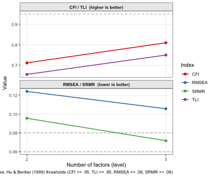
The shape of the trajectory matters as much as the absolute values. A sharp improvement from k = 2 to k = 3 suggests the third factor is capturing genuine signal. Flat or worsening indices suggest adding another level is splitting noise.
The examples in this vignette stop at k_max = 3 on
purpose, so the ESEM chunks build quickly and the tables stay legible.
The BFI hierarchy does not end there. For these data
suggest_k() points to roughly k = 5 (see
vignette("ackwards-suggest-k")), so a real analysis would
extend the trajectory further and read the fit curve across all five
levels. The truncated plot here shows the mechanics of reading
a fit trajectory, not the recommended depth for the BFI.
glance() also carries the deepest-level fit for quick
inspection:
glance(x_esem)
#>   engine rotation        cor k_max n_obs deepest_converged n_edges       CFI
#> 1   esem  varimax polychoric     3   875                 3       8 0.8098533
#>         TLI     RMSEA       SRMR BIC
#> 1 0.7498069 0.1055573 0.07172502  NA
Should you care about fit in a bass-ackwards workflow?
It depends on your goal:
- Exploratory (finding the hierarchical structure): fit is a secondary check. Start with PCA for speed, confirm with EFA or ESEM. If a level’s fit is poor, consider whether you have too many factors at that depth, or whether the items at that level are genuinely multidimensional.
-
Confirmatory / publication: fit is table-stakes for
ESEM or EFA. Report per-level CFI, TLI, RMSEA (and SRMR for ESEM)
alongside the hierarchy. The wide table and
autoplot(what = "fit")are designed for this. - Ordinal data: WLSMV (ESEM) gives fit indices appropriate for categorical items. EFA’s RMSEA/TLI under Pearson correlation is a rougher diagnostic.
The bottom line: per-level fit qualifies each level of the hierarchy. It does not bless the hierarchy as a whole. Use it to decide how deep the structure is credibly resolved, not to claim the overall model is “good”.
How much do the edges differ?
The primary output of bass-ackwards analysis is the between-level edges. For well-structured, continuous data, all three engines should agree closely on the hierarchy.
The table below compares the primary-parent edge strength for every adjacent level transition. The Δ column is the shift in connection strength (|EFA| − |PCA|). It is a direct, sign-safe measure of how much the latent-variable model changes your inference about the hierarchy.
| Primary-parent edges: PCA vs EFA | ||||
| From | To |
Edge strength (r)
|
||
|---|---|---|---|---|
| PCA | EFA | Δ (EFA − PCA)1 | ||
| m1f1 | m2f1 | 0.89 | 0.91 | 0.02 |
| m1f1 | m2f2 | 0.46 | 0.42 | −0.04 |
| m2f1 | m3f1 | 0.87 | 0.89 | 0.02 |
| m2f2 | m3f2 | 0.99 | 0.98 | −0.01 |
| m2f1 | m3f3 | 0.48 | 0.44 | −0.04 |
| 1 NA in either column means the engines disagree on the primary parent for that factor. | ||||
The r values are very close between engines. The hierarchy that PCA reveals is in effect the same hierarchy that EFA reveals. This convergence across methods is reassuring. It suggests the structure is real and not an artifact of the extraction method.
How clean this convergence looks depends on how strong the underlying
structure is. The simulated sim16 dataset
(?sim16) is an idealized case. Its planted 1 → 2 →
4 hierarchy is strong enough that engines and suggest_k()
criteria agree almost perfectly. Real data is messier. For
bfi25 the suggest_k() criteria span k = 4 to 6
even though the engines agree on the edges. Treat clean cross-method
consensus as the best case, not the norm. The
vignette("ackwards-suggest-k") develops this
idealized-versus-realistic contrast in full.
When the engines disagree on edges, that is itself informative. It usually indicates factors whose definition depends on whether you account for measurement error (EFA/ESEM) or not (PCA).
Choosing an engine
| Situation | Recommendation |
|---|---|
| Exploratory, large k, unknown structure | Start with "pca"
|
| Report a hierarchy with per-level fit (RMSEA/TLI) |
"efa", a complete reporting engine |
| You specifically need loading SEs / CIs (especially smaller n) | "esem" |
| Ordinal items and you want the field-standard WLSMV estimator |
"esem" with cor = "polychoric"
|
| Missing data you want handled by true FIML |
"esem" (ML/MLR) or PCA/EFA with
missing = "fiml"
|
Replicating Goldberg (2006) or
psych::bassAckward()
|
"pca" (the default engine. fm applies only
to "efa") |
A practical workflow: start with PCA to get a feel for the hierarchy and choose k. EFA is enough to confirm and report. It returns loadings, variance, edges, and per-level RMSEA/TLI. Reach for ESEM only when you need one of the three things it adds (loading SEs, WLSMV, or FIML). It is not a required “publication” upgrade. If PCA and EFA/ESEM edges agree, you have strong evidence for the hierarchy. If they disagree, investigate why.
Orthogonal or oblique rotation
The edges are correlations between factor scores at different levels, as implied by the correlation matrix the fit uses. The rotation you choose decides what a single edge means. Under varimax, the factors within each level are uncorrelated. So an edge from an ancestor to a descendant carries only their direct relationship. The correlation is the ancestor’s unique contribution, which is what lets the edges be drawn as a lineage diagram and summed, squared, into variance accounted for.
Under an oblique rotation, each level’s factors are allowed to correlate. That is often a more realistic model for one level taken on its own. But a between-level edge then becomes a total correlation. It mixes the direct ancestor and descendant relationship with overlap routed through the ancestor’s correlated neighbors at the same level. That quantity is meaningful, because it answers how strongly two constructs correlate. But it is no longer, by itself, a lineage statement. Thresholds tuned to varimax edges, such as the redundancy chase and the display cutoff, also read differently against it.
ackwards fits varimax by default. An oblique
rotation is available with rotation = "oblimin", or
"promax" for PCA and EFA, or "geomin" for
ESEM. With an oblique fit, the package reports the within-level factor
correlations beside the edges. It also labels the total correlation
r and the partialled coefficient beta
separately.
Varimax and oblimin on the same data
To see what changes, we fit EFA to the BFI-25 twice: once with the
default varimax rotation and once with oblimin. Both fits use the
polychoric basis and five levels. Oblimin rotates from random starts, so
the oblimin fit sets seed to make its result
repeatable.
x_var <- ackwards(bfi, k_max = 5, engine = "efa", cor = "polychoric")
x_obl <- ackwards(bfi,
  k_max = 5, engine = "efa", cor = "polychoric",
  rotation = "oblimin", seed = 1
)
#> ℹ Oblique rotation ("oblimin"): the factors within a level can correlate.
#> ℹ Each edge `r` is a total correlation, which includes overlap through
#>   correlated factors at the same level. Primary parents and signs use `r`, and
#>   `tidy(x)` reports the partialled `beta` beside it.
#> ! A factor's primary parent can then be a factor that only correlates with its
#>   real parent. Compare `r` with `beta` before reading a split as lineage.
#> ! The `cut_show` (0.3) and `prune()` `redundancy_r` conventions were calibrated
#>   under varimax.
The oblimin fit prints a message about what its edges mean. Each edge
r is now a total correlation. A factor’s primary parent can
be a factor that only correlates with its real parent. The display
cutoff was calibrated under varimax.
Within-level correlations. Under varimax, every factor correlation within a level is 0. Under oblimin, the factors correlate. The table below lists the oblimin correlations in order of absolute size, largest first.
fc <- tidy(x_obl, what = "factor_cor")
fc[order(-abs(fc$cor)), ]
#>    level factor_a factor_b         cor
#> 18     5     m5f3     m5f4  0.34080608
#> 3      3     m3f1     m3f3  0.33410491
#> 6      4     m4f1     m4f3  0.29972949
#> 15     5     m5f2     m5f3  0.24486305
#> 16     5     m5f2     m5f4  0.23701831
#> 11     5     m5f1     m5f2  0.23185860
#> 8      4     m4f2     m4f3  0.20810707
#> 1      2     m2f1     m2f2  0.20635837
#> 10     4     m4f3     m4f4  0.19750406
#> 17     5     m5f2     m5f5  0.19513178
#> 7      4     m4f1     m4f4  0.18722506
#> 20     5     m5f4     m5f5  0.18072108
#> 4      3     m3f2     m3f3  0.17521634
#> 2      3     m3f1     m3f2  0.17378293
#> 12     5     m5f1     m5f3  0.16359251
#> 5      4     m4f1     m4f2  0.14542884
#> 19     5     m5f3     m5f5  0.12100926
#> 13     5     m5f1     m5f4  0.03212687
#> 14     5     m5f1     m5f5 -0.02933486
#> 9      4     m4f2     m4f4  0.01362744
The largest is .34, between m5f3 and m5f4 at level 5. The next two are .33 between m3f1 and m3f3, and .30 between m4f1 and m4f3. We use those two below.
Matching the factors. A factor ID such as
m5f2 numbers a factor within its level, so the same ID can
name different factors in two fits. Before we compare the two
hierarchies, we match each oblimin factor to the varimax factor with the
most similar loadings. Tucker’s congruence coefficient compares two
columns of loadings. A value near 1 means the same pattern. We pick the
match by absolute size and keep the sign, so a factor that one fit flips
shows a negative value.
loading_matrix <- function(x, k) {
  d <- tidy(x, what = "loadings")
  unclass(xtabs(loading ~ item + factor, data = d[d$level == k, ]))
}
matches <- do.call(rbind, lapply(1:5, function(k) {
  cong <- psych::factor.congruence(
    loading_matrix(x_obl, k), loading_matrix(x_var, k),
    digits = 3
  )
  best <- apply(abs(cong), 1, which.max)
  data.frame(
    level = k,
    oblimin = rownames(cong),
    varimax = colnames(cong)[best],
    congruence = cong[cbind(seq_along(best), best)]
  )
}))
stopifnot(!anyDuplicated(matches$varimax)) # one-to-one
matches
#>    level oblimin varimax congruence
#> 1      1    m1f1    m1f1      1.000
#> 2      2    m2f1    m2f1      0.997
#> 3      2    m2f2    m2f2      0.992
#> 4      3    m3f1    m3f1      0.982
#> 5      3    m3f2    m3f2      0.994
#> 6      3    m3f3    m3f3      0.983
#> 7      4    m4f1    m4f1      0.982
#> 8      4    m4f2    m4f2      0.991
#> 9      4    m4f3    m4f3      0.981
#> 10     4    m4f4    m4f4      0.988
#> 11     5    m5f1    m5f1      0.974
#> 12     5    m5f2    m5f3      0.981
#> 13     5    m5f3    m5f2      0.943
#> 14     5    m5f4    m5f4      0.975
#> 15     5    m5f5    m5f5      0.986
Each oblimin factor matches a different varimax factor, so the match
is one to one at every level. Every congruence is positive, so no factor
is flipped. The IDs agree at levels 1 to 4. At level 5 the two fits
number two factors the other way round: oblimin’s m5f2 matches varimax’s
m5f3, and oblimin’s m5f3 matches varimax’s m5f2. The smallest congruence
is .94, for oblimin’s m5f3. That is far above the next value in its row
(.31). But it is just under .95, the value that prune()
uses by default on EFA fits when it judges two factors redundant. So
read this pair as a close match, not as one factor.
Primary parents. The next table translates the
oblimin primary edges into varimax IDs and joins them to the varimax
primary edges. The columns from and to hold
varimax IDs. The columns from_obl and to_obl
hold the oblimin IDs of the matched factors.
to_var <- setNames(matches$varimax, matches$oblimin)
p_var <- tidy(x_var, primary_only = TRUE)[, c("from", "to", "r")]
p_obl <- tidy(x_obl, primary_only = TRUE)[, c("from", "to", "r", "beta")]
names(p_obl) <- paste0(names(p_obl), "_obl")
p_obl$from <- unname(to_var[p_obl$from_obl])
p_obl$to <- unname(to_var[p_obl$to_obl])
tree <- merge(p_var, p_obl, by = c("from", "to"), all = TRUE)
print(tree, digits = 2)
#>    from   to    r from_obl to_obl r_obl beta_obl
#> 1  m1f1 m2f1 0.91     m1f1   m2f1  0.95     0.95
#> 2  m1f1 m2f2 0.42     m1f1   m2f2  0.51     0.51
#> 3  m2f1 m3f1 0.89     m2f1   m3f1  0.93     0.93
#> 4  m2f1 m3f3 0.44     m2f1   m3f3  0.65     0.62
#> 5  m2f2 m3f2 0.98     m2f2   m3f2  0.99     1.00
#> 6  m3f1 m4f1 1.00     m3f1   m4f1  1.00     1.02
#> 7  m3f2 m4f2 0.99     m3f2   m4f2  0.99     0.99
#> 8  m3f3 m4f3 0.83     m3f3   m4f3  0.91     0.89
#> 9  m3f3 m4f4 0.54     m3f3   m4f4  0.58     0.60
#> 10 m4f1 m5f2 0.82     m4f1   m5f3  0.84     0.85
#> 11 m4f1 m5f4 0.57     m4f1   m5f4  0.80     0.79
#> 12 m4f2 m5f1 1.00     m4f2   m5f1  0.99     0.99
#> 13 m4f3 m5f3 0.98     m4f3   m5f2  0.98     0.97
#> 14 m4f4 m5f5 0.99     m4f4   m5f5  0.99     0.98
anyNA(tree)
#> [1] FALSE
Every varimax primary edge has an oblimin edge between the matched
factors, and no row is left without a partner. After the match, the two
fits draw the same primary-parent tree. Under oblimin, beta
is a regression weight and not a correlation, so it can pass 1. It does
for m3f1 → m4f1 (1.02), and for m2f2 → m3f2 (1.002), which the table
rounds to 1.00.
Secondary edges. A secondary edge is any edge that
is not a primary edge. The function below lists the secondary edges that
reach the display cutoff (above_cut, at the default
cut_show of 0.3).
above_cut_secondary <- function(x) {
  e <- tidy(x)
  e[e$above_cut & !e$is_primary, c("from", "to", "r", "beta")]
}
above_cut_secondary(x_var)
#> [1] from to   r    beta
#> <0 rows> (or 0-length row.names)
above_cut_secondary(x_obl)
#>    from   to         r        beta
#> 11 m3f1 m4f3 0.3294898 0.015582657
#> 22 m4f1 m5f2 0.3040742 0.001471389
#> 34 m4f3 m5f4 0.3395477 0.156271630
Varimax has no secondary edge above the cutoff. Oblimin has three,
with r from .30 to .34, and all three beta
values are positive. For two of them, beta is close to
zero: .016 for m3f1 → m4f3 and .0015 for m4f1 → m5f2. Holding the other
factors at the from level constant leaves almost no weight
on these two edges. The primary parent of m4f3 is m3f3, which correlates
.33 with m3f1. In oblimin IDs, the primary parent of m5f2 is m4f3, which
correlates .30 with m4f1. The third edge, m4f3 → m5f4, keeps a
beta of .16. The primary parent of m5f4 is m4f1, which
correlates .30 with m4f3. Holding m4f1 and the other level-4 factors
constant cuts this edge from .34 to .16. Part of the edge is shared with
those factors, and part is not.
Diagrams. The two figures draw each fit with
autoplot(). The oblimin diagram shows the three secondary
edges, and the varimax diagram shows none. The two diagrams also place
some factors in a different order within a row.
autoplot(x_var)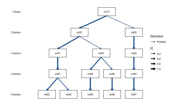
EFA with varimax rotation.
autoplot(x_obl)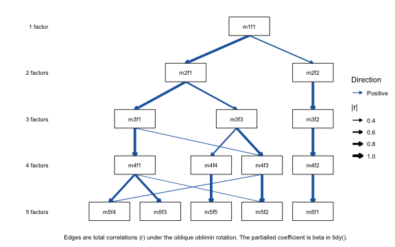
EFA with oblimin rotation.
How to decide
If your question is the hierarchy, meaning what splits into what and
how strongly, keep varimax. If your question is the structure of a
single level on its own terms, an oblique fit answers it. Read its edges
as total correlations, and use beta for claims about a
factor’s unique lineage. The primary parents, the sign alignment, and
the diagram still use r under every rotation.
Missing data
ackwards() accepts a missing argument that
controls how incomplete rows are handled before the correlation matrix,
engine fit, and edges are computed. The full per-engine semantics,
including the minor ESEM ML/MLR pairwise fit-versus-edges inconsistency
and the $meta fields that record it, are documented in
?ackwards. In brief:
-
"pairwise"(default): all available observations, pairwise. MCAR-valid, full N. Warns when NAs are present. -
"listwise": complete cases only, applied before all steps, so the correlation matrix, fit, and edges are fully consistent. Valid for all engines. -
"fiml": full-information ML, on two routes. Forengine = "esem"(withestimator = "ML"or"MLR"andcor = "pearson"), lavaan estimates under FIML and the edges derive from its FIML saturated model. Forengine = "pca"or"efa"on the Pearson basis, the correlation matrix is estimated bypsych::corFiml()(full-information ML under multivariate normality, MAR-valid) and fed to the usualW′RWbetween-level algebra. The route announces itself with a message.missing = "fiml"errors for WLSMV/ULSMV (limited-information estimators have no FIML extension). It also errors for a non-Pearson basis on any engine, becausecorFiml()and lavaan’s FIML each estimate a multivariate-normal matrix. FIML improves estimation but does not impute items, sokeep_scores = TRUEstill yieldsNAfor incomplete rows.
FIML for continuous PCA/EFA
For continuous data with MAR missingness, pass
missing = "fiml" directly. It is more principled than
pairwise deletion, which is only MCAR-valid:
# sim16 is continuous, so FIML's normality assumption is appropriate here.
set.seed(1)
sim_na <- sim16
for (j in seq_len(ncol(sim_na))) sim_na[sample(nrow(sim_na), 60L), j] <- NA

x_fiml <- ackwards(sim_na, k_max = 4, engine = "efa", missing = "fiml")
#> ℹ `missing = "fiml"`: correlation matrix estimated via `psych::corFiml()`
#>   (full-information ML).
#> ℹ Fit indices use N = 1000 (`n_obs = "total"`); point estimates (loadings,
#>   edges) are unaffected by this choice.
#> ! Fit indices are approximate: a FIML correlation matrix is fed into a
#>   normal-theory EFA (a two-step procedure). See `?ackwards` (`n_obs`).
x_fiml
#>
#> ── Bass-Ackwards Analysis (ackwards) ───────────────────────────────────────────
#> Engine: efa
#> Rotation: varimax
#> Basis: pearson
#> n: 1,000
#> k (max): 4
#>
#> ── Levels ──
#>
#> ✔ k = 1: 1 factor, 23.3% variance
#> ✔ k = 2: 2 factors, 38.7% variance
#> ✔ k = 3: 3 factors, 48.2% variance
#> ✔ k = 4: 4 factors, 56.8% variance
#>
#> ── Edges ──
#>
#> 9 of 20 edges have |r| ≥ 0.3
#> ────────────────────────────────────────────────────────────────────────────────
#> Note: This is a series of linked solutions, not a fitted hierarchical model.
#> Cross-level edges are descriptive score correlations. Per-level fit indices
#> (EFA/ESEM) describe how well a k-factor model fits the items at that level --
#> they do not validate the edges or the hierarchy itself.
Under the hood this estimates the correlation matrix with
psych::corFiml() and runs the normal W′RW
algebra on it. So the loadings and edges are exactly what the manual
ackwards(psych::corFiml(sim_na), …) correlation-matrix call
would give. That seam remains
available for non-standard cases, e.g. a FIML matrix you have already
computed elsewhere.
Two caveats matter. First, the fit-index N is your
call. FIML draws information from every partially observed row,
so there is no single “correct” N for the EFA fit indices, and the
n_obs argument selects it on this route.
"total" is the default: every row contributing to the FIML
likelihood, the convention a FIML analysis reports. It is mildly
anti-conservative, because χ² and RMSEA then treat partial rows
as if complete. "complete" (the complete-case count) is
conservative. The loading and edge point estimates are
unaffected by this choice. Only the fit indices depend on it,
and those are approximate under this two-step route (FIML matrix into
normal-theory EFA) regardless of N. Second, the route assumes
multivariate normality, so it is for
continuous data only. For ordinal items use
engine = "esem" with cor = "polychoric"
instead.
Which option to use?
| Situation | Recommendation |
|---|---|
| Continuous data, little missingness |
"pairwise" (default) |
| Ordinal data + WLSMV, any missingness |
"pairwise" (uses available.cases,
MCAR-valid, full N) |
| Want consistent fit statistics and edges (continuous ML/MLR) | "listwise" |
| ESEM ML/MLR, meaningful missingness, want all rows used in estimation | "fiml" |
| Continuous PCA/EFA, MAR missingness |
"fiml" (via
psych::corFiml(). See above) |
| MAR-valid with ordinal (not yet built-in) | MI via lavaan.mi or mirt
|
Correlation-matrix input
You may have a pre-computed correlation matrix: a published table, a
polychoric matrix computed externally, a FIML estimate for missing data,
or a subset you want to analyse without refitting. You can pass it
directly to ackwards() or suggest_k(). The
matrix is auto-detected from its shape (square, symmetric, unit
diagonal).
R <- cor(bfi25, use = "pairwise.complete.obs")

# PCA from a correlation matrix (n_obs optional for PCA; required for EFA)
x_R <- ackwards(R, k_max = 5)
# EFA requires n_obs for fit indices:
x_efa_R <- ackwards(R, k_max = 5, engine = "efa", n_obs = 875L)

# Edges are identical to the raw-data run (same W'RW algebra):
x_d <- ackwards(bfi25, k_max = 5)
all.equal(tidy(x_R)$r, tidy(x_d)$r) # TRUE within floating-point tolerance
Constraints
| Constraint | Detail |
|---|---|
| Engine |
"pca" and "efa" only. "esem"
errors (lavaan needs raw data) |
n_obs |
Required for "efa". Optional for "pca"
(stored as NA) |
cor argument |
Ignored (basis is fixed). Warns if set explicitly |
missing argument |
Ignored. Warns if set explicitly |
| Factor scores |
keep_scores = TRUE, augment(),
tidy(what = "scores") all error |
$cor field |
Stored as NA. Shown as
"(user-supplied matrix)" in print |
suggest_k() with a correlation matrix
sk_R <- suggest_k(R, n_obs = 875L)
# CD is skipped (resampling requires raw item distributions)
# PA, MAP, and VSS run normally
Performance with many items (ESEM)
Bass-ackwards analyses often involve large item pools. ESEM is the
most expensive engine because it fits a separate lavaan
model at every level. Two automatic optimisations keep this
manageable:
-
Sample statistics are computed once. For ordinal
data (
cor = "polychoric", WLSMV), lavaan’s thresholds, polychoric matrix, and asymptotic weight matrix depend only on the data, not on the number of factors. Soackwards()computes them at the first level and reuses them for every deeper level. This is the single biggest saving at large item counts. -
Levels can be fit in parallel. The per-level fits
are independent. Install
future.applyand set a future plan before your call. The default plan is sequential (no change in behaviour).
library(future)
plan(multisession, workers = 4) # parallel across background R sessions

x <- ackwards(items, k_max = 8, engine = "esem", cor = "polychoric", seed = 1)

plan(sequential) # restore when done
plan() comes from future (it is
not re-exported by future.apply), so load
future directly rather than reaching for
future.apply::plan(). Parallelism pays off only when the
per-level fits are genuinely heavy. For small problems the worker
startup cost can outweigh the gain. Results are reproducible across
plans when you pass seed. PCA and EFA compute their
correlation matrix once and do not need this.
You may only need the hierarchy (loadings and edges) and not ESEM’s
rotation-aware standard errors and per-level fit indices. In that case
engine = "efa" with cor = "polychoric"
computes the polychoric matrix once and runs psych::fa() at
each level. That is substantially cheaper than k WLSMV fits, and it
recovers the same structure.
References
Asparouhov, T., & Muthén, B. (2009). Exploratory structural equation modeling. Structural Equation Modeling, 16(3), 397–438.
Goldberg, L. R. (2006). Doing it all Bass-Ackwards: The development of hierarchical factor structures from the top down. Journal of Research in Personality, 40(4), 347–358.
Hu, L., & Bentler, P. M. (1999). Cutoff criteria for fit indexes in covariance structure analysis: Conventional criteria versus new alternatives. Structural Equation Modeling, 6(1), 1–55.
Waller, N. G. (2007). A general method for computing hierarchical component structures by Goldberg’s Bass-Ackwards method. Journal of Research in Personality, 41(4), 745–752.