
The Forbes Extension: Skip-Level Connections and Pruning
Source:vignettes/ackwards-forbes.Rmd
ackwards-forbes.RmdThe classic Goldberg (2006) method computes between-level factor-score correlations only for adjacent levels: 1↔︎2, 2↔︎3, 3↔︎4, and so on. A factor is an unobserved dimension that explains why a set of items correlate, and a factor score is each person’s estimated position on a factor. Forbes (2023) extended the method in two ways. Her method computes correlations across all level pairs, not only adjacent ones, and it uses those extra connections to identify and flag redundant or artifactual factors in the hierarchy. A redundant factor restates a factor at another level rather than refining it. An artifactual factor is a by-product of the extraction rather than a construct in the data.
This vignette covers both extensions: pairs = "all" and
prune. It teaches the concepts on a small didactic dataset.
For a full reproduction of the paper’s 155-variable applied example on
the bundled forbes2023 dataset, see
vignette("ackwards-forbes2023").
The limitation of adjacent-only edges
An adjacent-only hierarchy shows you the immediate parent-child relationships. What it cannot tell you is whether a factor at level k is in substance the same construct as a factor several levels up. That would be a sign that the intermediate levels are adding noise rather than resolution.
Consider a factor that appears at k = 2, k = 3, and k = 4 and correlates > 0.97 with its counterpart at every adjacent level. The adjacent-only diagram shows three consecutive arrows, each nearly perfect. But nothing in the diagram directly flags that the k = 3 factor is redundant. You could skip straight from k = 2 to k = 4 without losing any information.
Skip-level correlations make this visible by computing the correlation between every pair of levels, not only neighbors.
Computing every between-level correlation with
pairs = "all"
Adding pairs = "all" extends the edge table from
adjacent pairs only to every combination of levels.
# Classic adjacent-only
x_adj <- ackwards(bfi, k_max = 5, cor = "polychoric")

# All pairs
x_all <- ackwards(bfi, k_max = 5, cor = "polychoric", pairs = "all")

# How many edges?
nrow(tidy(x_adj, what = "edges")) # adjacent only
#> [1] 40
nrow(tidy(x_all, what = "edges")) # all pairs
#> [1] 85
With k = 5, the adjacent-only model has 40 edges (1×2 + 2×3 + 3×4 + 4×5). The all-pairs model adds every non-adjacent pair (1↔︎3, 1↔︎4, 1↔︎5, 2↔︎4, 2↔︎5, 3↔︎5), for 85 edges total.
Reading the skip-level edge table
The table below keeps the non-adjacent edges (levels more than one
apart) with |r| >= 0.5, strongest first. It is drawn
from tidy(x_all, what = "edges"):
| Strongest skip-level edges (|r| ≥ 0.5, non-adjacent levels) | ||||
| Sorted by |r|; shows at most 12 rows | ||||
| From | To | Level (from) | Level (to) | r |
|---|---|---|---|---|
| m3f2 | m5f2 | 3 | 5 | 0.98 |
| m2f2 | m4f2 | 2 | 4 | 0.97 |
| m2f2 | m5f2 | 2 | 5 | 0.97 |
| m2f1 | m4f1 | 2 | 4 | 0.85 |
| m3f1 | m5f1 | 3 | 5 | 0.82 |
| m1f1 | m3f1 | 1 | 3 | 0.77 |
| m1f1 | m4f1 | 1 | 4 | 0.75 |
| m3f3 | m5f3 | 3 | 5 | 0.73 |
| m2f1 | m5f1 | 2 | 5 | 0.69 |
| m3f3 | m5f5 | 3 | 5 | 0.68 |
| m1f1 | m5f1 | 1 | 5 | 0.61 |
| m3f1 | m5f4 | 3 | 5 | 0.56 |
Several factors connect across two or more levels with correlations above 0.90. m3f2 (level 3, factor 2) correlates 0.98 with m5f2 (level 5, factor 2), jumping two levels. This tells you that m3f2 and m5f2 are in substance the same construct. The intermediate levels are just refinements within a stable dimension.
Reading the strongest edge with care
Reading the strongest edge off a table of many correlations is itself a form of selection. With k = 5 the all-pairs table holds 85 edges, and the maximum of that many correlations is biased upward even when every individual estimate is honest. Treat a “strongest link” claim as descriptive rather than inferential. If it is load-bearing, pre-specify which pair of factors you care about rather than reporting whichever correlation came out largest.
Pruning: identifying redundant factors
The prune() verb uses the skip-level correlations to
automatically flag factors that may not be adding genuine information to
the hierarchy.
Chains of near-identical factors with
prune(x, "redundant")
A redundant chain is a sequence of factors connected by near-perfect correlations (|r| ≥ 0.9 by default) across levels. Suppose m2f2 → m3f2 → m4f2 → m5f1 all share r > 0.97. The chain reaches the deepest level, so its bottom node m5f1, the most specific and best-defined manifestation, is retained. The others (m2f2, m3f2, m4f2) are flagged as redundant: they repeat rather than refine the same dimension. A chain that stops short of the deepest level instead keeps its top node, the broadest manifestation (Forbes, 2023).
By default (redundancy_criterion = "direct") the
criterion is a star anchored on the chain’s deepest
factor, not a walk. Every candidate ancestor is judged by its
own score correlation directly with that deepest leaf. The
chain forms while each shallower factor correlates
|r| ≥ 0.9 with the leaf, which means it shares at least 81%
of its variance with the leaf directly. This is the rule Forbes’s own
code uses, and the honest reading of “the same construct”. Two things it
is not. It does not require each consecutive pair to
correlate (that adjacent-hop rule is
redundancy_criterion = "adjacent"), and it does not screen
every ancestor pair against every other. Because correlation is
non-transitive, the star and the adjacent-hop walk can disagree in deep
hierarchies. An ancestor can join on a strong direct link to the leaf
even where its hop to the next chain member is weak. On a shallow
hierarchy like this one the two agree.
x_prune <- ackwards(bfi, k_max = 5, cor = "polychoric", pairs = "all") |>
  prune("redundant")
#> ℹ Redundancy pruning (direct criterion, |r| ≥ 0.9) flagged 6 nodes.
#> ℹ Nodes are retained in the object; inspect with `x$prune$nodes` and
#> `x$prune$chains`.| Node-level pruning annotation | |||
| 6 of 15 factors flagged as redundant | |||
| Factor | Level | Flagged? | Reason |
|---|---|---|---|
| m1f1 | 1 | FALSE | — |
| m2f1 | 2 | FALSE | — |
| m2f2 | 2 | TRUE | redundant |
| m3f1 | 3 | FALSE | — |
| m3f2 | 3 | TRUE | redundant |
| m3f3 | 3 | FALSE | — |
| m4f1 | 4 | TRUE | redundant |
| m4f2 | 4 | TRUE | redundant |
| m4f3 | 4 | TRUE | redundant |
| m4f4 | 4 | TRUE | redundant |
| m5f1 | 5 | FALSE | — |
| m5f2 | 5 | FALSE | — |
| m5f3 | 5 | FALSE | — |
| m5f4 | 5 | FALSE | — |
| m5f5 | 5 | FALSE | — |
6 factors are flagged as redundant (m2f2, m3f2, m4f1, m4f2, m4f3, m4f4): 1 factor at k = 2, 1 factor at k = 3, the entire k = 4 level. This is a striking finding. For this dataset and this k, the four-factor level adds little beyond what you already know from k = 3 and k = 5.
The flagged factors are not removed from the object.
prune() is purely a diagnostic annotation, not a deletion.
You can still inspect their loadings (a loading is the correlation
between an item and a factor), use their scores, and include them in the
diagram. Pruning flags guide interpretation. They do not alter the
model.
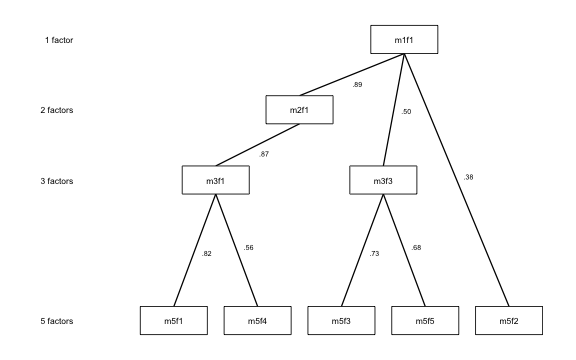
The pruned-factor diagram
For presentations and publications it is cleaner to omit the flagged
factors entirely. Each retained factor then connects directly to its
single strongest kept ancestor, even when that ancestor is several
levels away. This is the Forbes (2023) pruned-factor diagram, activated
by drop_pruned = TRUE.
Forbes (2023) presents two variants: one with correlation labels on each arrow and one without. The first is useful when the strength of each spanning connection matters to the interpretation. The second is cleaner for presentations. Both are reproduced below using the same publication style: black lines, uniform width, plain line ends, and no legend.
With correlation labels
(show_r = TRUE):
autoplot(x_prune,
  drop_pruned = TRUE, show_r = TRUE,
  color_pos = "black", color_neg = "black",
  edge_linewidth = 0.6, show_arrows = FALSE, legend = FALSE
)
Without labels (cleaner for slides or when the exact values are not the focus):
autoplot(x_prune,
  drop_pruned = TRUE,
  color_pos = "black", color_neg = "black",
  edge_linewidth = 0.6, show_arrows = FALSE, legend = FALSE
)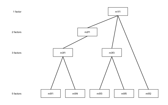
Level 4 is entirely pruned, leaving a visible gap in the y-axis. The
gap is intentional: it shows which level was removed. Spanning
arrows bridge directly from level 3 factors to level 5 factors (and from
level 2 to level 5 where intermediate levels were flagged). In this
publication style every drawn line has the same uniform weight
(edge_linewidth = 0.6). Only connections with |r| at or
above the display threshold (cut_show, default 0.3) are
drawn at all.
To close the gaps and compact the layout while retaining the original level numbers on the axis:
autoplot(x_prune,
  drop_pruned = TRUE, compress_levels = TRUE,
  color_pos = "black", color_neg = "black",
  edge_linewidth = 0.6, show_arrows = FALSE, legend = FALSE
)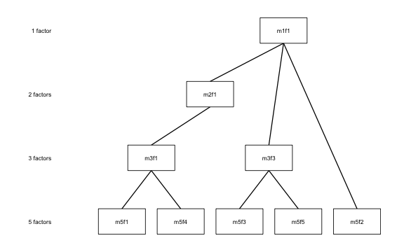
The level labels still read “1 factor”, “2 factors”, “3 factors”, “5 factors”, so readers know which levels were retained. The uniform vertical spacing makes the diagram easier to read in constrained page layouts.
For further cosmetic customization (colours, node labels, arrowheads,
and more) see vignette("ackwards-visualization").
Inspecting structural similarity with
prune(x, "artifact")
An artifact factor is one that looks like a copy of a factor from another level rather than a genuine refinement. Its loading pattern closely resembles a factor elsewhere in the hierarchy. Similarity is measured by Tucker’s congruence coefficient (φ), which compares two columns of loadings item by item and returns 1 when they are proportional:
φ ranges from −1 to +1. Values above 0.95 are conventionally read as near-identical loading patterns regardless of sign (Lorenzo-Seva & ten Berge, 2006).
Unlike "redundant", the artifact mode never
drops anything automatically. The reason is not that flagging
would add investigator degrees of freedom. A standardized flag that is
always computed the same way removes researcher discretion
rather than adding it. The reason is that the decision to drop
a factor as an artifact is substantive: Forbes (2023) is explicit that
identifying an artifact requires researcher judgment. So
prune(x, "artifact") computes and stores the evidence for
you to weigh, and leaves the drop decision to you. The evidence
is Tucker’s φ for every cross-level factor pair in
x$prune$phi, plus the structural signals of the next
section in x$prune$structural.
x_art <- ackwards(bfi, k_max = 5, cor = "polychoric", pairs = "all") |>
  prune("artifact")
#> ℹ Artifact mode: Tucker's φ computed for all cross-level factor pairs.
#> ℹ Structural signals computed: 2 factors flagged (few_items / orphan /
#>   split_merge).
#> ℹ Near-redundant band: 5 cross-level pairs just below the redundancy thresholds
#>   (|r| in [0.8, 0.9)).
#> ℹ Inspect `x$prune$phi`, `x$prune$structural`, and `x$prune$near_redundant`;
#>   removal is a researcher judgment (Forbes, 2023).
The table to read is x$prune$phi. The natural first cut
is the non-adjacent pairs with the highest |φ|. A deep
factor whose loading pattern nearly duplicates a factor two or more
levels up is the classic candidate:
| Strongest non-adjacent loading congruences | ||||
| Top 8 pairs by |φ|, from x$prune$phi — evidence, not flags | ||||
| From | To | Level (from) | Level (to) | φ |
|---|---|---|---|---|
| m3f2 | m5f2 | 3 | 5 | 0.99 |
| m2f2 | m4f2 | 2 | 4 | 0.98 |
| m2f2 | m5f2 | 2 | 5 | 0.98 |
| m2f1 | m4f1 | 2 | 4 | 0.93 |
| m3f1 | m5f1 | 3 | 5 | 0.92 |
| m1f1 | m3f1 | 1 | 3 | 0.88 |
| m1f1 | m4f1 | 1 | 4 | 0.86 |
| m2f1 | m5f1 | 2 | 5 | 0.85 |
For these data the strongest non-adjacent congruence is |φ| = 0.99.
Values near 1 mean the deeper factor recycles an earlier loading
pattern. But a congruence this high travels with a near-perfect
score correlation too, so these top pairs are already the province of
prune(x, "redundant"). The factor they name is flagged (and
dropped from the publication diagram) by the redundancy rule above. The
distinctive contribution of artifact mode is not re-flagging what
redundancy already caught. It is surfacing the messier band just
below the redundancy thresholds.
The near-redundant band
Full redundancy, |r| ≥ redundancy_r, is dropped in the
redundancy stage. Forbes (2023) uses the artifact flags mainly for the
pairs that sit just under that line. A pair that correlates,
say, |r| = 0.89 and shares a loading pattern
φ = 0.94 is not quite redundant. A rotation re-orients the
factors within a level without changing how well they fit. Such a pair
is a candidate for re-rotation, worth a second look rather than a clean
new level of resolution. The function prune(x, "artifact")
collects exactly these in x$prune$near_redundant. It keeps
every cross-level pair that is not itself fully
redundant yet is close to redundant on either signal. Close means within
near_margin (default 0.1) below the
threshold. The first signal is the pair’s direct score correlation
|r|. Off PCA (principal component analysis, which
summarizes the items with weighted sums called components), the pair’s
Tucker φ is a second signal, judged against its own
threshold. One signal in its window is enough.
#> ℹ Redundancy pruning (direct criterion, |r| ≥ 0.9) flagged 6 nodes.
#> ℹ Nodes are retained in the object; inspect with `x$prune$nodes` and
#> `x$prune$chains`.| Near-redundant band | |||||
| Cross-level pairs just below the redundancy thresholds — evidence, not flags | |||||
| From | To | Level (from) | Level (to) | r | φ |
|---|---|---|---|---|---|
| m1f1 | m2f1 | 1 | 2 | 0.89 | 0.94 |
| m2f1 | m3f1 | 2 | 3 | 0.87 | 0.94 |
| m2f1 | m4f1 | 2 | 4 | 0.85 | 0.93 |
| m4f1 | m5f1 | 4 | 5 | 0.84 | 0.93 |
| m3f1 | m5f1 | 3 | 5 | 0.82 | 0.92 |
The strongest near-redundant pair here is m1f1 ↔︎ m2f1 (r = 0.89, φ =
0.94) and, unlike the top-φ pairs above, neither factor is flagged by
prune(x, “redundant”): this pair is a genuine near-miss, not something
redundancy already drops. The examples here use the default PCA engine,
so redundancy_phi is NULL and only the
|r| band is active. On an EFA or ESEM fit
redundancy_phi auto-resolves to 0.95 and the
φ band switches on too (prune() announces
this). EFA (exploratory factor analysis) models the items as a small
number of shared factors plus item-specific noise. ESEM (exploratory
structural equation modeling) fits that same factor model in lavaan and
adds standard errors. Widen or narrow the band with
near_margin. Like the φ table, the band is
report-only: no factor is dropped on its basis.
The two modes surface different fingerprints of the same underlying question:
-
"redundant": this factor appears at multiple levels with near-identical score correlations. It persists unchanged as k increases. Auto-flagged (with Forbes’s retention rule), because the score-correlation chain is a sharp, replicable criterion. -
"artifact": this factor’s loading pattern closely resembles a factor elsewhere in the hierarchy, or its structure looks under-identified (next section). Reported only. The call is yours.
Structural artifact signals
Congruence (φ) is not the only fingerprint of an artifactual factor.
Forbes (2023, Fig. 2) describes several structural signatures,
and prune(x, "artifact") reports three of them per factor
in x$prune$structural:
-
few_items: the factor is the primary (highest-loading) home for fewer thanmin_itemsitems (default3). A factor anchored by one or two items is under-identified and often an extraction artifact rather than a replicable construct. -
orphan: the factor’s strongest correlation to the immediately neighbouring levels is beloworphan_r(default0.5). It does not connect to the solutions on either side, so it does not replicate across the hierarchy. -
split_merge: the factor’s primary items were spread across two or more different parent factors at the level above. Items that were separated at the coarser solution have been merged under one factor at the finer solution. This is the split-then-merge anomaly of Forbes Fig. 2.
| Structural artifact signals | ||||
| 2 of 15 factors raise a structural signal | ||||
| Factor | Level | Few items | Orphan | Split/merge |
|---|---|---|---|---|
| m1f1 | 1 | FALSE | FALSE | FALSE |
| m2f1 | 2 | FALSE | FALSE | FALSE |
| m2f2 | 2 | FALSE | FALSE | FALSE |
| m3f1 | 3 | FALSE | FALSE | FALSE |
| m3f2 | 3 | FALSE | FALSE | FALSE |
| m3f3 | 3 | FALSE | FALSE | TRUE |
| m4f1 | 4 | FALSE | FALSE | FALSE |
| m4f2 | 4 | FALSE | FALSE | FALSE |
| m4f3 | 4 | FALSE | FALSE | FALSE |
| m4f4 | 4 | FALSE | FALSE | TRUE |
| m5f1 | 5 | FALSE | FALSE | FALSE |
| m5f2 | 5 | FALSE | FALSE | FALSE |
| m5f3 | 5 | FALSE | FALSE | FALSE |
| m5f4 | 5 | FALSE | FALSE | FALSE |
| m5f5 | 5 | FALSE | FALSE | FALSE |
Like Tucker’s φ, these signals are flag-and-report
only: prune() never removes a factor on their
basis. As before, a standardized signal removes researcher
discretion rather than adding it. What requires judgment is the
substantive decision to treat a factor as an artifact, which
the signals only point you toward. The two thresholds,
min_items and orphan_r, are arguments to
prune().
Tuning the thresholds
The redundancy criterion has an adjustable redundancy_r
threshold (default 0.90) matching Forbes (2023). The
artifact criterion has no auto-flag threshold.
prune(x, "artifact") computes Tucker’s φ for researcher
inspection, and no factors are auto-flagged.
The redundancy_phi companion criterion.
Redundancy can optionally require that linked factors also share a
loading pattern (Tucker’s φ above a threshold), not only a high score
correlation. The redundancy_phi argument controls this, and
its default (NULL) auto-resolves based on the
engine:
-
PCA: no φ filter. Component scores are
determinate. Unlike factor scores they are exact linear
functions of the observed data. So the score correlation
|r|is the correlation between the components themselves, under the correlation matrix the fit uses, and it suffices as the redundancy signal. -
EFA / ESEM: φ is required to exceed
0.95(Lorenzo-Seva & ten Berge, 2006). Factor scores are indeterminate: any factor admits infinitely many score series consistent with the model. That makes an|r|-only rule too liberal, and the loading-congruence guard makes the criterion conservative.prune()announces this auto-resolution in the console.
The examples here use the default PCA engine, so no φ filter is
applied. To disable the φ guard on an EFA/ESEM run, pass
redundancy_phi = NA. To set your own threshold, pass a
number in (0, 1].
For the BFI, the result is the same across a wide range of thresholds because the redundant chains all have correlations > 0.97. The flagging is unambiguous. With your own data you may find borderline cases where the threshold matters.
Because prune() is a cheap, standalone step, checking a
few redundancy_r thresholds does not require refitting
ackwards() each time. The already-fit x_all
object is re-pruned directly:
thresholds <- c(0.80, 0.85, 0.90, 0.95)
counts <- sapply(thresholds, function(thr) {
  x <- prune(x_all, "redundant", redundancy_r = thr)
  sum(tidy(x, what = "nodes")$pruned)
})
#> ℹ Redundancy pruning (direct criterion, |r| ≥ 0.8) flagged 9 nodes.
#> ℹ Nodes are retained in the object; inspect with `x$prune$nodes` and
#>   `x$prune$chains`.
#> ℹ Redundancy pruning (direct criterion, |r| ≥ 0.85) flagged 8 nodes.
#> ℹ Nodes are retained in the object; inspect with `x$prune$nodes` and
#>   `x$prune$chains`.
#> ℹ Redundancy pruning (direct criterion, |r| ≥ 0.9) flagged 6 nodes.
#> ℹ Nodes are retained in the object; inspect with `x$prune$nodes` and
#>   `x$prune$chains`.
#> ℹ Redundancy pruning (direct criterion, |r| ≥ 0.95) flagged 6 nodes.
#> ℹ Nodes are retained in the object; inspect with `x$prune$nodes` and
#>   `x$prune$chains`.
thr_df <- data.frame(redundancy_r = thresholds, n_flagged = counts)| Factors flagged redundant at each redundancy_r threshold | |
| redundancy_r | Factors flagged |
|---|---|
| 0.80 | 9 |
| 0.85 | 8 |
| 0.90 | 6 |
| 0.95 | 6 |
For the BFI all thresholds agree: the flagged factors are clearly redundant, not borderline cases. In noisier datasets or smaller samples you will typically see the count increase as you lower the threshold.
Practical interpretation
The Forbes extension does not change the core bass-ackwards analysis. It enriches it with two questions:
Do any factors persist unchanged across multiple levels? (
pairs = "all") Skip-level correlations near 1.0 indicate stable dimensions that survive changes in k. These are exactly the kind of stable construct you want to report.Are there levels where the factor structure is just reorganizing rather than genuinely differentiating? (
prune(x, "redundant")) Flagged levels can often be removed from the k range without losing interpretive content.
A common workflow: fit with pairs = "all" first to
examine the full picture, then pipe the result through
prune(x, "redundant") to identify which levels add the most
new information. Use that to guide your focus in reporting. For where
redundancy pruning sits in the full recommended workflow, see
vignette("ackwards-girard"). That workflow also gates
hierarchy depth on split-half replicability with
comparability(), which checks whether each factor
re-emerges in repeated random half-splits of the sample.
References
Forbes, M. K. (2023). Improving hierarchical models of individual differences: An extension of Goldberg’s bass-ackward method. Psychological Methods. https://doi.org/10.1037/met0000546
Goldberg, L. R. (2006). Doing it all Bass-Ackwards: The development of hierarchical factor structures from the top down. Journal of Research in Personality, 40(4), 347–358.
Lorenzo-Seva, U., & ten Berge, J. M. F. (2006). Tucker’s congruence coefficient as a meaningful index of factor similarity. Methodology, 2(2), 57–64. https://doi.org/10.1027/1614-2241.2.2.57
Tucker, L. R. (1951). A method for synthesis of factor analysis studies (Personnel Research Section Report No. 984). Department of the Army.