


Bass-ackwards hierarchical structural analysis in R
ackwards implements Goldberg’s (2006) bass-ackwards method and its modern extensions for mapping the hierarchical structure of multivariate data.
The core idea is this. Instead of asking how many factors best describe your data, ask how the solutions at different levels of detail relate to one another. A factor is a summary variable that stands in for a group of items that tend to move together. A 1-factor solution captures the broadest shared variance. A 5-factor solution captures narrower, more specific dimensions. Bass-ackwards analysis traces how broad factors split into narrow ones. It also shows which narrow factors are only re-combinations of broader ones.
The package supports three extraction engines. PCA (principal component analysis) summarizes the items with weighted sums called components. EFA (exploratory factor analysis) instead models the items as caused by latent factors plus item-specific noise. ESEM (exploratory structural equation modeling) fits the same kind of factor model inside a structural equation framework, which adds fit indices and standard errors. After extraction each engine applies a rotation, which re-orients the factors without changing how well they fit. By default the package uses varimax, which pushes each item toward one factor and keeps the factors uncorrelated. An oblique rotation, which lets the factors within a level correlate, is an option. Ordinal data are items with a few ordered categories, such as a 1 to 5 rating. For such data the package can use polychoric correlations, which estimate the correlation between the continuous traits assumed to underlie the ordered responses.
Beyond fitting, the package is a full analysis toolkit. suggest_k() brackets the plausible depth of the hierarchy. comparability() gates that depth on split-half replicability. That is, it checks whether each factor re-emerges when the sample is split into two random halves. Forbes’s (2023) prune() flags redundant factors (factors that persist across levels without changing) and artifactual factors from the connections between non-adjacent levels. boot_edges() puts bootstrap confidence intervals on every edge. predict() scores new observations out of sample.
Installation
Install the released version from CRAN:
install.packages("ackwards")Or the development version from GitHub:
# install.packages("pak")
pak::pak("jmgirard/ackwards")
Quick start
We use bfi25, the built-in 25-item Big Five example dataset (see ?bfi25 for provenance). Its items are recorded on a 6-point ordinal scale, so we set cor = "polychoric". We also fit the dataset directly rather than removing incomplete rows first, so its built-in IPIP item labels flow through to top_items().
Step 1: Suggest a range of k
suggest_k() runs five complementary criteria to help you choose an upper bound for the hierarchy depth. Two of them are forms of parallel analysis, which compares the eigenvalues of your data against those of random data with the same shape. The others are MAP, VSS, and optionally Comparison Data.
sk
#>
#> ── Factor / Component Count Suggestion (ackwards) ──────────────────────────────
#> Variables: 25
#> n: 1,000
#> Basis: pearson
#> Tested k: 1-8
#>
#> ── Criteria (k = 1-8) ──
#>
#>   k  PA-PC  PA-FA      MAP    VSS-1    VSS-2  CD
#>   1     ✔︎      ✔︎   0.0246   0.5121   0.0000   ✔︎
#>   2     ✔︎      ✔︎   0.0190   0.5761   0.6636   ✔︎
#>   3     ✔︎      ✔︎   0.0172   0.5969   0.7288   ✔︎
#>   4     ✔︎      ✔︎   0.0164   0.6198*  0.7781   ✔︎
#>   5     ✔︎      ✔︎   0.0160*  0.5730   0.7912*  ✔︎
#>   6     -      ✔︎   0.0170   0.5592   0.7530   ✔︎
#>   7     -      -   0.0201   0.5698   0.7290   ✔︎*
#>   8     -      -   0.0231   0.5615   0.7252   -
#>   ✔︎ retained   * optimal k   - not retained
#>
#> ── Recommendations ──
#>
#> • PA-PC: k <= 5
#> • PA-FA: k <= 6
#> • MAP: k = 5
#> • VSS-1: k = 4
#> • VSS-2: k = 5
#> • CD: k = 7
#> Consensus range: k = 4-7
#> ────────────────────────────────────────────────────────────────────────────────
#> Note: k_max in ackwards() is a maximum depth. Setting k_max one or two levels
#> above the consensus to observe factor fragmentation is intentional.
#> Caution: PA-PC tends to overextract; structures may not replicate (Forbes,
#> 2023). PA-FA and CD are more conservative. Use the range.
The criteria converge on a consensus range that covers k = 5, consistent with the known Big Five structure of this instrument.
Step 2: Fit the hierarchy
ackwards() fits factor models at every level from 1 to k_max. It then computes the correlations between the factor scores of different levels, and those correlations define the hierarchy. By default it correlates neighbouring levels only. A factor score is each person’s estimated standing on a factor, computed from their item responses. Each correlation comes from the scoring weights and the correlation matrix the fit uses, and it is exact for that matrix. With a polychoric matrix, as here, scores computed from the items do not in general reproduce the edges exactly. The result is a set of linked solutions whose edges are score correlations, never a fitted hierarchical model.
x <- ackwards(bfi25, k_max = 5, cor = "polychoric", missing = "listwise")
x
#>
#> ── Bass-Ackwards Analysis (ackwards) ───────────────────────────────────────────
#> Engine: pca
#> Rotation: varimax
#> Basis: polychoric
#> n: 875
#> k (max): 5
#>
#> ── Levels ──
#>
#> ✔ k = 1: 1 factor, 23.2% variance
#> ✔ k = 2: 2 factors, 35.5% variance
#> ✔ k = 3: 3 factors, 44.6% variance
#> ✔ k = 4: 4 factors, 52.2% variance
#> ✔ k = 5: 5 factors, 58.4% variance
#>
#> ── Edges ──
#>
#> 14 of 40 edges have |r| ≥ 0.3
#> ────────────────────────────────────────────────────────────────────────────────
#> Note: This is a series of linked solutions, not a fitted hierarchical model.
#> Cross-level edges are descriptive score correlations. Per-level fit indices
#> (EFA/ESEM) describe how well a k-factor model fits the items at that level --
#> they do not validate the edges or the hierarchy itself.
Step 3: Visualize
autoplot() draws the hierarchical diagram. Each row is a level, with k = 1 at the top and k = 5 at the bottom. Arrows connect each narrow factor to the broad factor it inherits from. Arrow thickness encodes the size of the correlation and colour encodes its sign, and both are legended. The visualization vignette covers the encodings, direction = "horizontal", and the rest of the styling.
autoplot(x)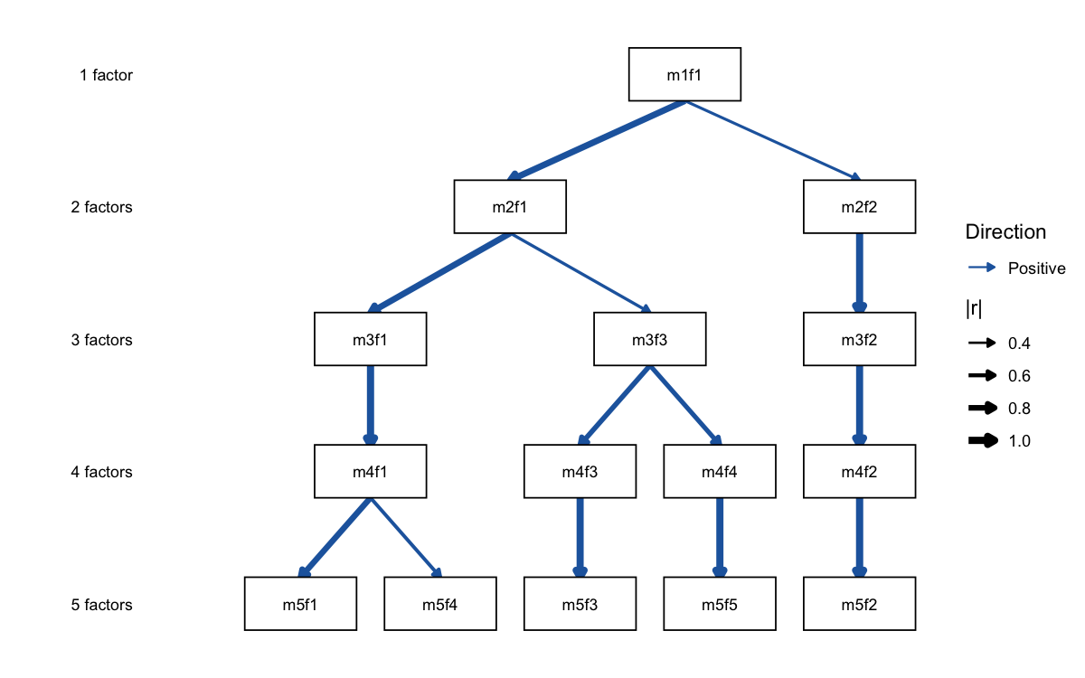
The five-factor level cleanly splits into the Big Five. The single broad factor at k = 1 (roughly general positive character) differentiates first into positive vs. negative affect (k = 2), then into successively narrower traits.
Step 4: Interpret and score
top_items() lists each factor’s salient items, printed with the built-in IPIP labels of bfi25, so you can read what a factor means. An item is salient when its loading, the correlation between the item and the factor, is large. augment() turns the hierarchy into factor scores for downstream analysis.
# What does each of the five factors mean? (salient items, |loading| >= 0.5)
top_items(x, level = 5, cut = 0.5)
#>
#> ── Salient items by factor (ackwards) ──────────────────────────────────────────
#> Engine: pca
#> Cut: |loading| >= 0.5
#> Top-n: all
#>
#> ── Level 5 (5 factors) ──
#>
#> m5f1
#> E2: Find it difficult to approach others [-0.752]
#> E4: Make friends easily [0.747]
#> E1: Don't talk a lot [-0.701]
#> E3: Know how to captivate people [0.677]
#> E5: Take charge [0.597]
#>
#> m5f2
#> N3: Have frequent mood swings [-0.825]
#> N1: Get angry easily [-0.810]
#> N2: Get irritated easily [-0.805]
#> N5: Panic easily [-0.688]
#> N4: Often feel blue [-0.646]
#>
#> m5f3
#> C2: Continue until everything is perfect [0.735]
#> C4: Do things in a half-way manner [-0.716]
#> C1: Am exacting in my work [0.690]
#> C3: Do things according to a plan [0.679]
#> C5: Waste my time [-0.652]
#>
#> m5f4
#> A1: Am indifferent to the feelings of others [-0.704]
#> A3: Know how to comfort others [0.703]
#> A2: Inquire about others' well-being [0.692]
#> A5: Make people feel at ease [0.580]
#> A4: Love children [0.522]
#>
#> m5f5
#> O5: Will not probe deeply into a subject [-0.705]
#> O3: Carry the conversation to a higher level [0.655]
#> O1: Am full of ideas [0.604]
#> O2: Avoid difficult reading material [-0.595]
#> O4: Spend time reflecting on things [0.551]
#> ────────────────────────────────────────────────────────────────────────────────
#> Loadings reflect primary-parent sign alignment. Use tidy(x, what = "loadings")
#> for the full matrix.Beyond the basics
A serious analysis rarely stops at one fit. Three verbs turn the hierarchy from a picture into a defensible result, and one scores new data:
-
comparability(bfi25, k_max = 6)gates hierarchy depth on split-half replicability. It finds the deepest level at which every factor re-emerges in random halves of the sample (Everett 1983, Saucier et al. 2005). -
prune(x, "redundant")flags factors that persist across levels without differentiating, which is the redundancy question of Forbes (2023). -
boot_edges(x, bfi25)attaches bootstrap confidence intervals to every between-level edge. -
predict(x, newdata)scores observations the model never saw, in the training metric, which is the standard cross-validation pattern.
The recommended-workflow vignette strings these into a six-step analysis.
Learn more
| Vignette | Topic |
|---|---|
| Introduction | The basics end-to-end: suggest_k to ackwards to summarize, plot, interpret, and score |
| Recommended workflow | Replicability-gated hierarchies: gate depth on split-half comparability()
|
| Choosing k | Five criteria explained: pros and cons, bias direction, engine pairing |
| Forbes extension | Skip-level edges, redundancy pruning, pairs = "all"
|
| Engines & rotation | When to choose EFA or ESEM over PCA, with convergence and loading comparison |
| Ordinal data | Polychoric correlations, attenuation bias, and WLSMV estimation |
| Interpreting & labeling |
top_items(), hierarchy-aware naming, label_template() round-trip |
| Visualization | Styling autoplot(): sign and magnitude encoding, layout orientation, labels, publication figures |
Citation
If you use ackwards in your research, please cite the package:
citation("ackwards")
#> To cite package 'ackwards' in publications use:
#>
#>   Girard J (2026). _ackwards: Bass-Ackwards Hierarchical Structural
#>   Analysis_. R package version 0.2.0.9000,
#>   <https://github.com/jmgirard/ackwards>.
#>
#> A BibTeX entry for LaTeX users is
#>
#>   @Manual{,
#>     title = {ackwards: Bass-Ackwards Hierarchical Structural Analysis},
#>     author = {Jeffrey M. Girard},
#>     year = {2026},
#>     note = {R package version 0.2.0.9000},
#>     url = {https://github.com/jmgirard/ackwards},
#>   }
Please also cite the relevant method paper(s). Cite Goldberg (2006) https://doi.org/10.1016/j.jrp.2006.01.001 for the bass-ackwards method itself. Cite Forbes (2023) https://doi.org/10.1037/met0000546 if you use the extended method (pairs = "all", redundancy or artifact pruning).